 SARS-CoV-2 Duotang
Duotang, a genomic epidemiology analyses and mathematical modelling notebook
CAMEO
01 June, 2026
Citation
If you use the VirusSeq Data Portal or Duotang resource, please cite: Gill et al. (2024) Microbial Genomics. doi:10.1099/mgen.0.001293
SARS-CoV-2 In Canada
Introduction
This notebook was built to explore Canadian SARS-CoV-2 genomic and epidemiological data with the aim of investigating viral evolution and spread. It is developed by the CAMEO team (Computational Analysis, Modelling and Evolutionary Outcomes Group) for sharing with collaborators, including public health labs. These analyses are freely available and open source, enabling code reuse by public health authorities and other researchers for their own use.
Canadian genomic and epidemiological data will be regularly pulled from various public sources (see list below) to keep these analyses up-to-date. Only representations of aggregate data will be posted here.
Important limitations
These analyses represent only a snapshot of SARS-CoV-2 evolution in Canada. Only some infections are detected by PCR testing, only some of those are sent for whole-genome sequencing, and not all sequences are posted to public facing repositories. Furthermore, sequencing volumes and priorities have changed during the pandemic, specific variants or populations might be preferentially sequenced at certain times in certain jurisdictions. When possible, these differences in sampling strategies are mentioned but they are not always known. With the arrival of the Omicron wave, many jurisdictions across Canada reached testing and sequencing capacity mid-late December 2021 and thus switched to targeted testing of priority groups (e.g., hospitalized patients, health care workers, and people in high-risk settings). Currently, most jurisdictions are sequencing mainly hospitalized patients or outbreaks, with little population-level random sampling, underestimating case counts and viral diversity.
Thus, interpretation of these plots and comparisons between health regions should be made with caution, considering that the data may not be fully representative. These analyses are subject to frequent change given new data and updated lineage designations.
The last sample collection date is 19 April, 2026
Current SARS-CoV-2 situation
Cases (and genomic sampling) have been very low, involving primarily a combination of PQ subvariants (descended from NB.1.8.1), with some XFG subvariants, plus some BA.3.2 subvariants at lower levels While we continue to monitor, no current variant exhibits unusually fast growth.
Variants of current interest (due to their current/potential growth advantage, mutations of potential functional significance, or spread in other countries):
- NB.1.8.1 subvariants, including RC variants
- XFG subvariants, including subvariants of XFG.1.1
- PE.1.4
- BA.3.2 (including RE) subvariants, due in part to evidence they have disproportionately affected children. Also, this variant has been less detected in clinical cases verses wastewater.
We continue to monitor for, but have not recently detected, any other highly divergent variants in Canada (“saltation” lineages with a sudden increase in number of mutations).
Note reductions or delays in data can cause delays in the detection of new variants and more uncertainty when estimating selection.
We thank the global team of those monitoring variants (such as those posting issues here: https://github.com/cov-lineages/pango-designation/issues), and other SARS-CoV-2 genome analysis tool providers (see List of Useful Tools below), which play a key role in identifying new variants of note.
Sublineages in Canada
There are 256 unique named variants currently circulating in Canada since 2025-12-10 (last 120 days). Please see Pango lineage table for number of sequences per lineage present.
Below is an interactive visualization showing frequencies of ciruclating lineages, sub-divided by major sub-lineages, currently circulating in Canada. A table of lineage frequencies can be downloaded by clicking on the (Frequency Table Download) button.
Tips: Click and drag to zoom, double click to reset. Clicking on an item in the legend will hide it, double clicking an item in legend will hide everything else but that item.
Last 120 days
Last 120 days sublineages starting from 2025-12-10 (Frequency Table Download)
BA.1
BA.1 sublineages (Frequency Table Download)
BA.2
BA.2 sublineages (Frequency Table Download)
BA.4
BA.4 sublineages (Frequency Table Download)
BA.5
BA.5 sublineages (Frequency Table Download)
Recombinants
Recombinants sublineages (Frequency Table Download)
## [1] NA
## [1] NA
## [1] NASelection on recent variants
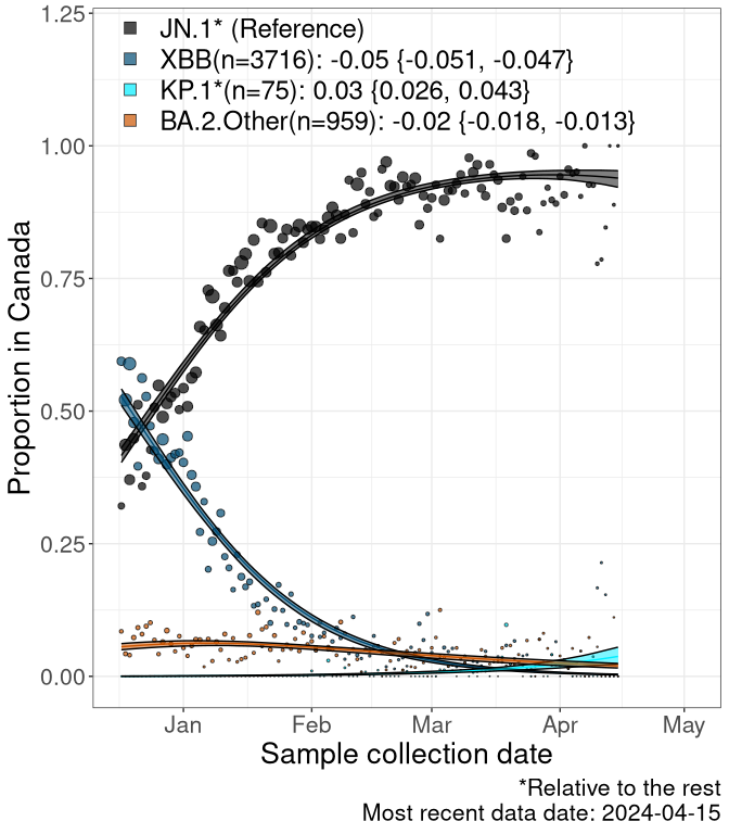
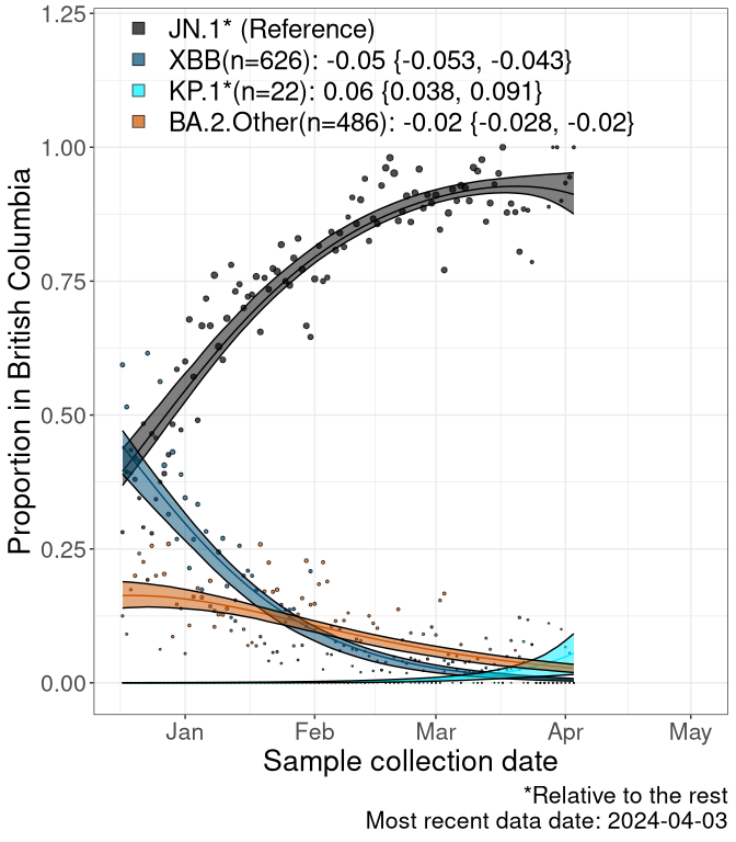
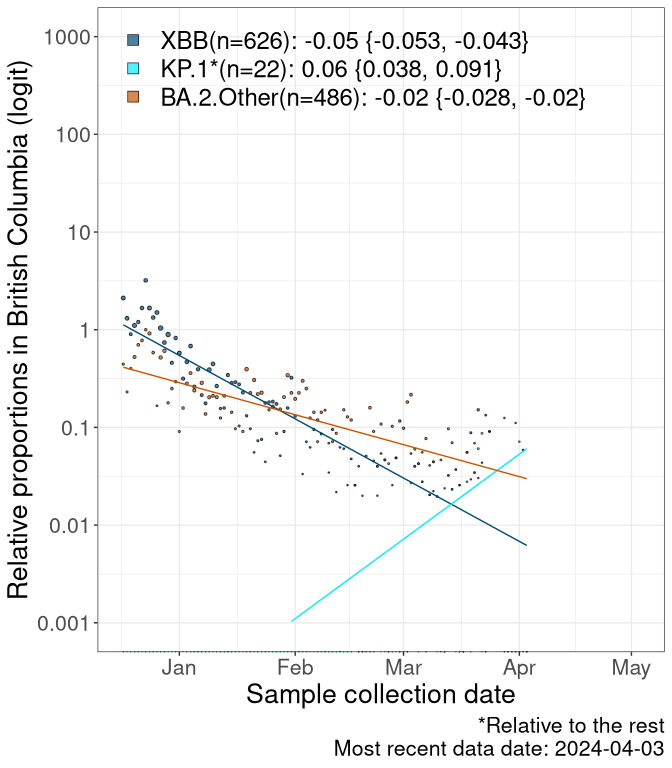
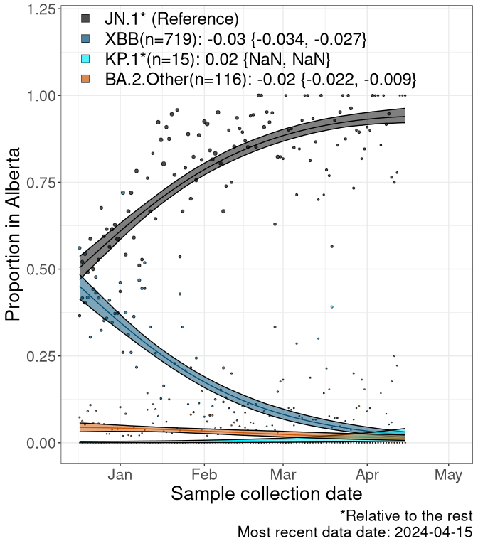
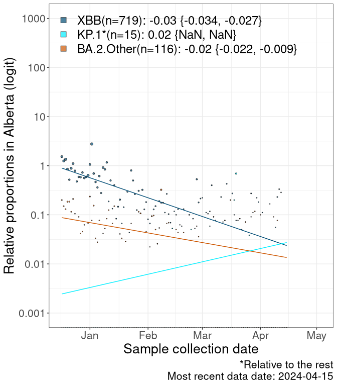
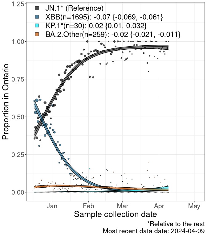
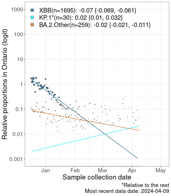
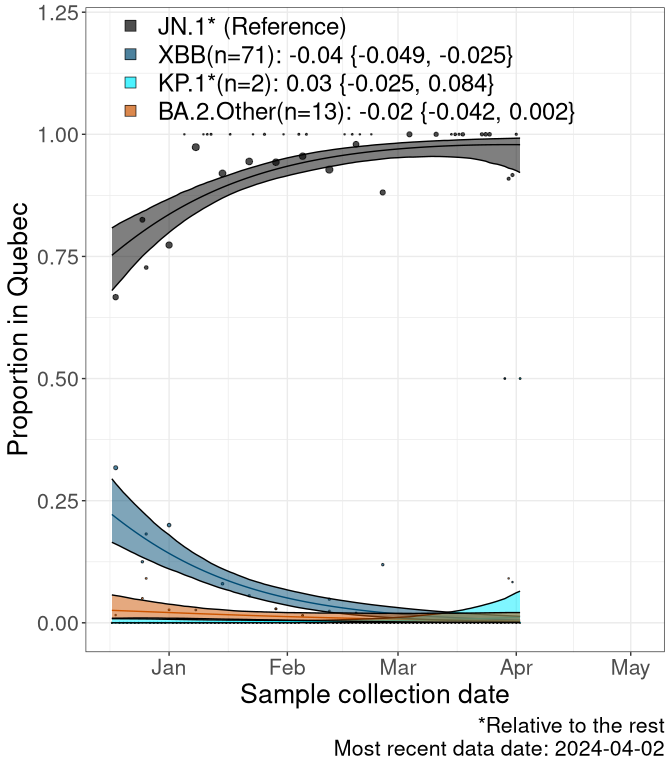
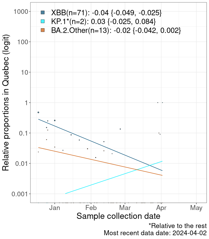
Here we examine the relative rate of spread of the different sublineages of SARS-CoV-2 currently circulating in Canada. Specifically, we determine if a new or emerging lineage has a selective advantage (s), and by how much, against a previously common reference lineage (broad scale (and in the Fastest Growing Lineages section): XFG* and at the fine scale, against XFG.3; see methods for more details about selection and how it is estimated).
Currently, the major group of SARS-CoV-2 lineages circulating are BA.2.86* variants. At the broad scale, we are now tracking the frequencies of XFG* (as the reference), NB, PQ and other BA.2 lineages (mainly BA.2.86 lineages).
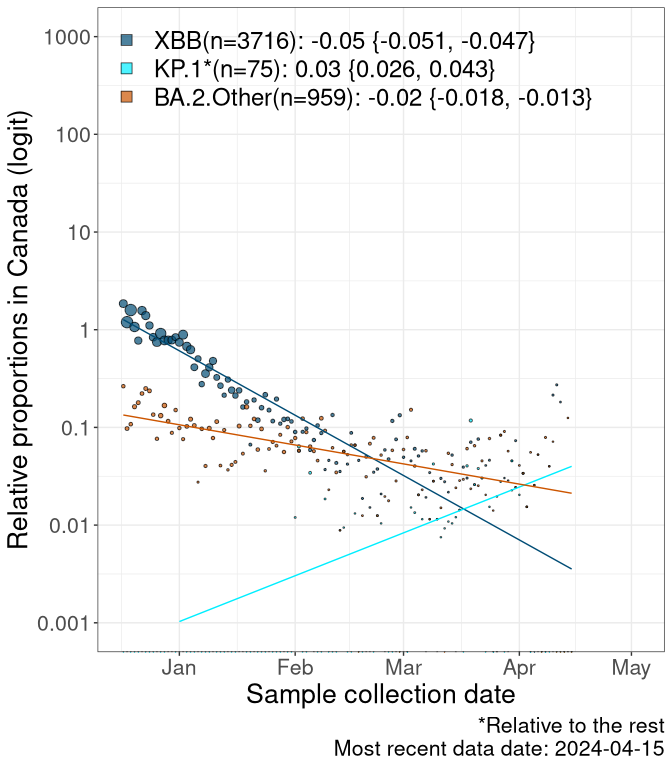
Left plot: y-axis is the proportion of these sub-lineages over time. Right plot: y-axis describes the logit function, log(freq(NB/PQ/Others)/freq(XFG*)), which gives a straight line whose slope is the selection coefficient if selection is constant over time (see methods).
For comparison, Alpha had a selective advantage of s ~ 6%-11% per day over preexisting SARS-CoV-2 lineages, and Delta had a selective advantage of about 10% per day over Alpha.
Caveat: These selection analyses must be interpreted with caution due to the potential for non-representative sampling, lags in reporting, and spatial heterogeneity in prevalence of different sublineages across Canada. Provinces that do not have at least 20 sequences of a lineage during this time frame are not displayed.
Canada
Canada
BC
British Columbia
AB
Alberta
SK
Saskatchawan


MB
Manitoba


ON
Ontario
QC
Quebec
NS
Nova Scotia

NB
New Brunswick


NL
Newfoundland and Labrador


NULL
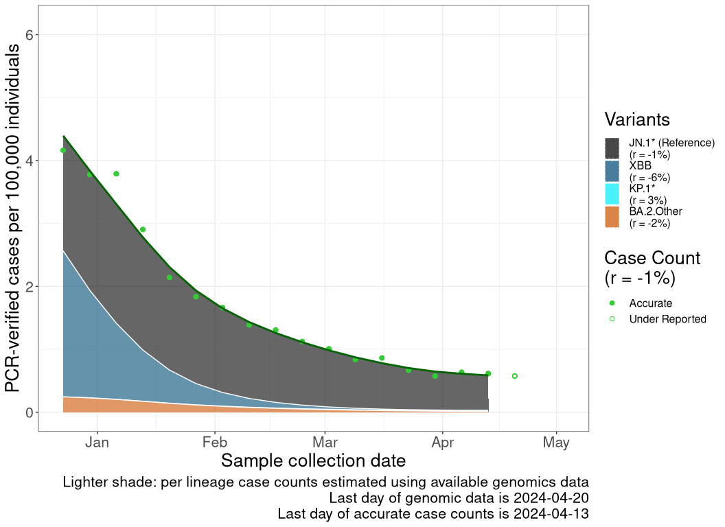
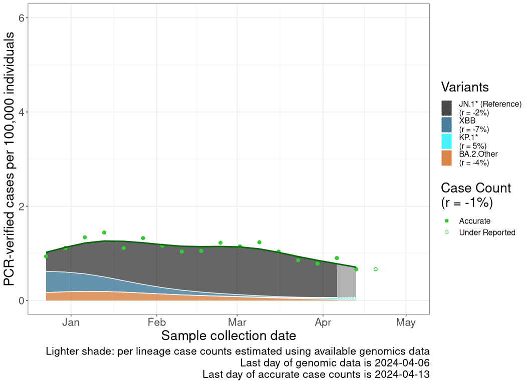
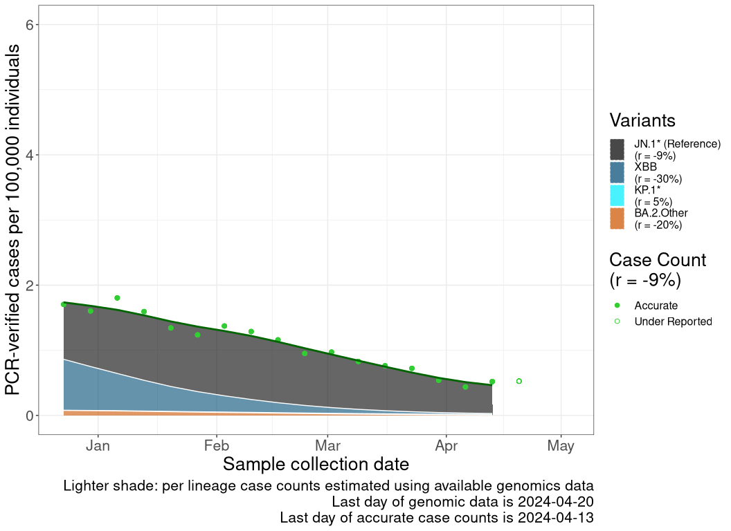
Detection trends by variant
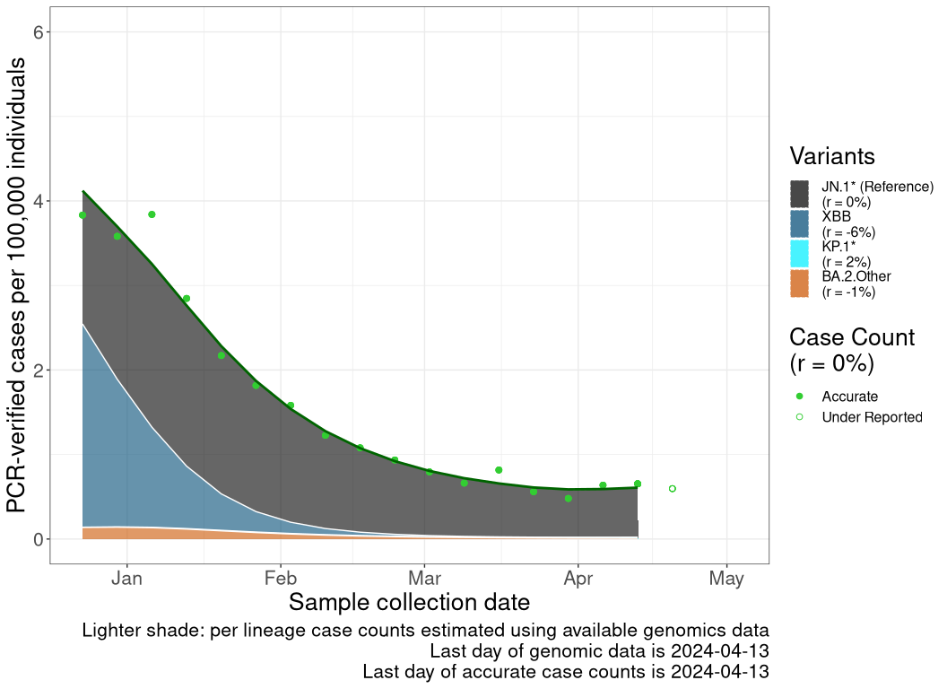
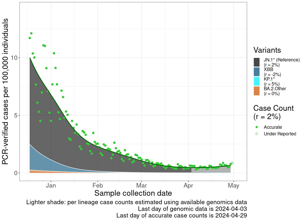
These plots follow the number of detected cases per 100,000 individuals (green dots), ignoring the most recent week (hollow circles), which is generally underestimated as data continue to be gathered. A cubic spline is fit to the log of these case counts to illustrate trends (top curve). The last two days of inferred case counts are then used to estimate the daily exponential growth rate r in COVID-19 cases. The fit from the “Selection on Omicron” section above is used to show how each of the sub-lineages is growing or shrinking, with the corresponding growth rate \(r\) for each sub-lineage on the last two days of inferred case counts. Note that only a small fraction of cases are currently being officially tested, so the y-axis height is underestimated by orders of magnitude (e.g., by 92-fold in BC mid-2022, Skowronski et al. 2022). Thus, graphs should only be used to describe growth trends and not absolute numbers. For detailed methodology including a change in case data source on 13 July 2024, please see the methods section in the appendix..
Canada
Canada
BC
British Columbia
AB
Alberta
SK
Saskatchawan

MB
Manitoba

ON
Ontario
QC
Quebec
NS
Nova Scotia

NB
New Brunswick

NL
Newfoundland and Labrador
NULL
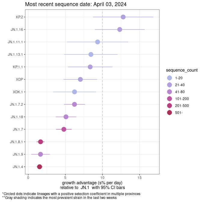
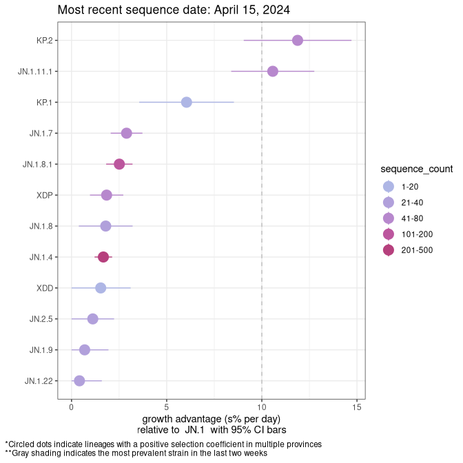
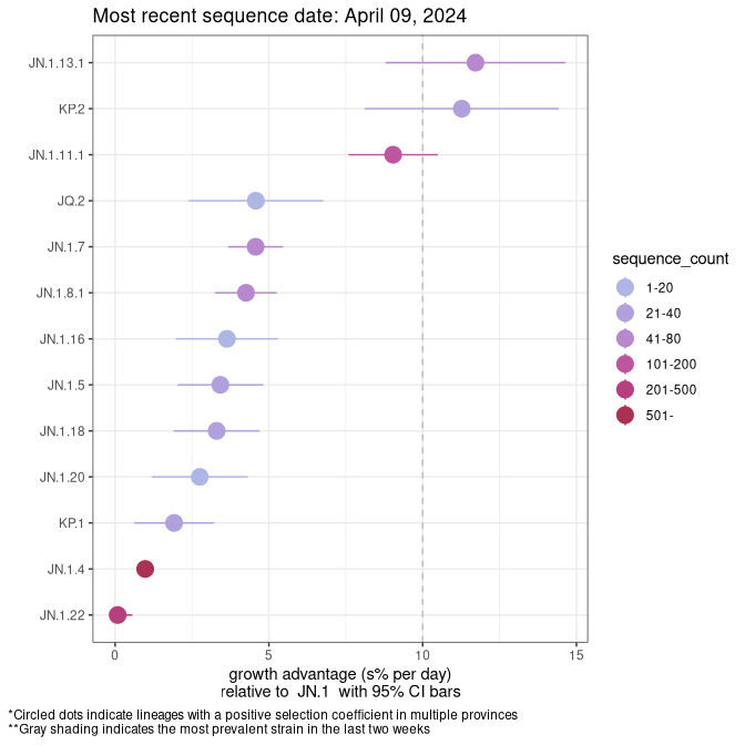
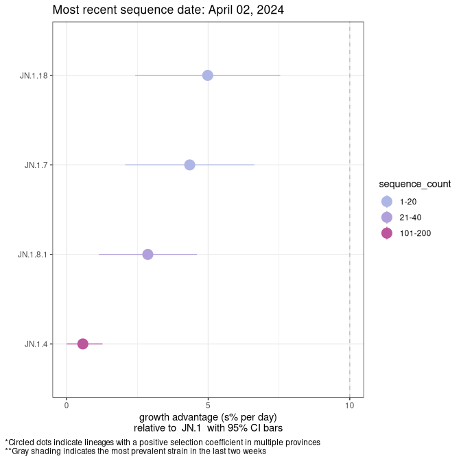
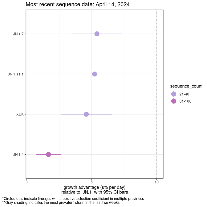
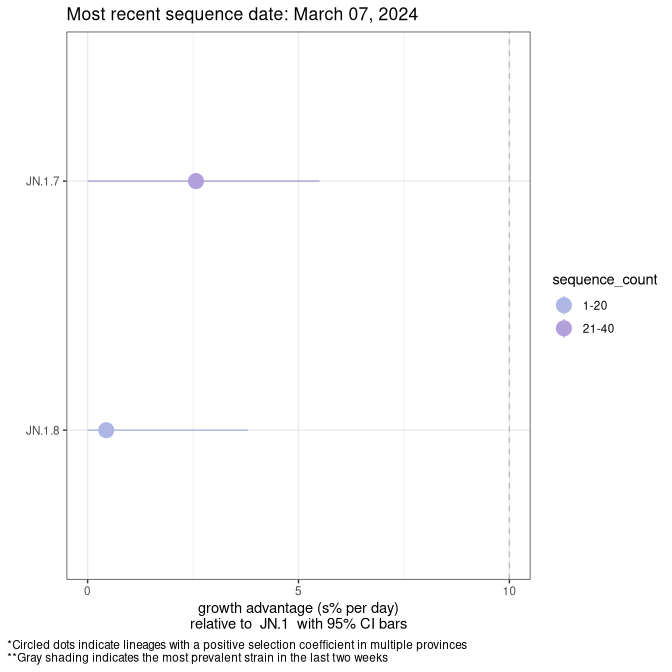
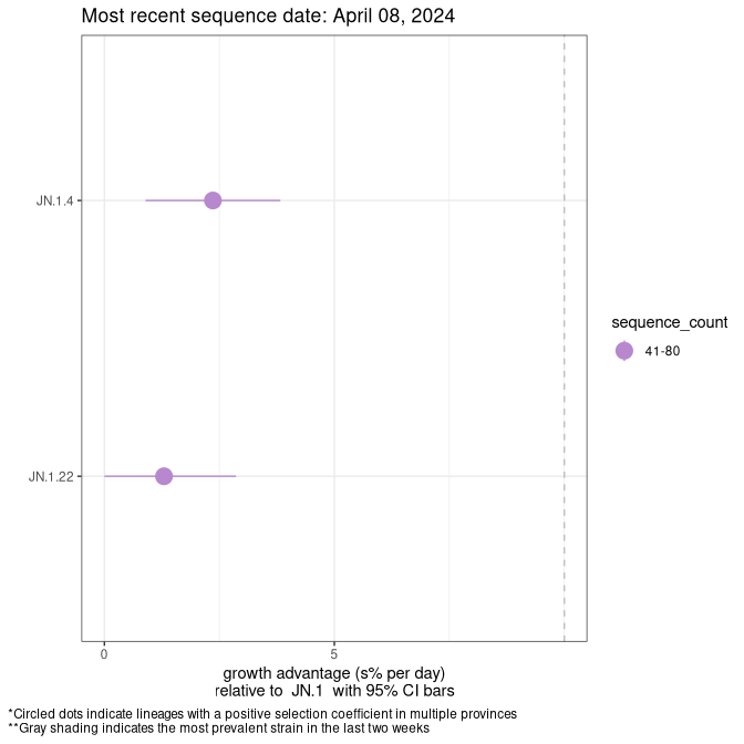
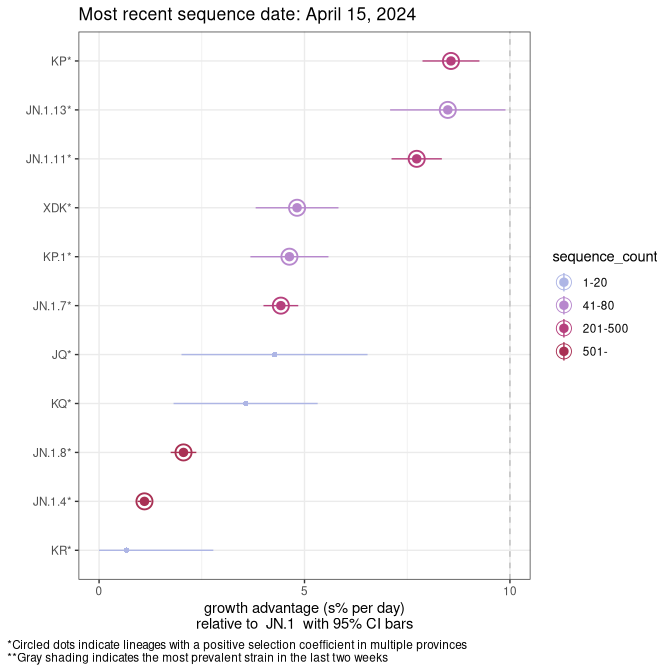
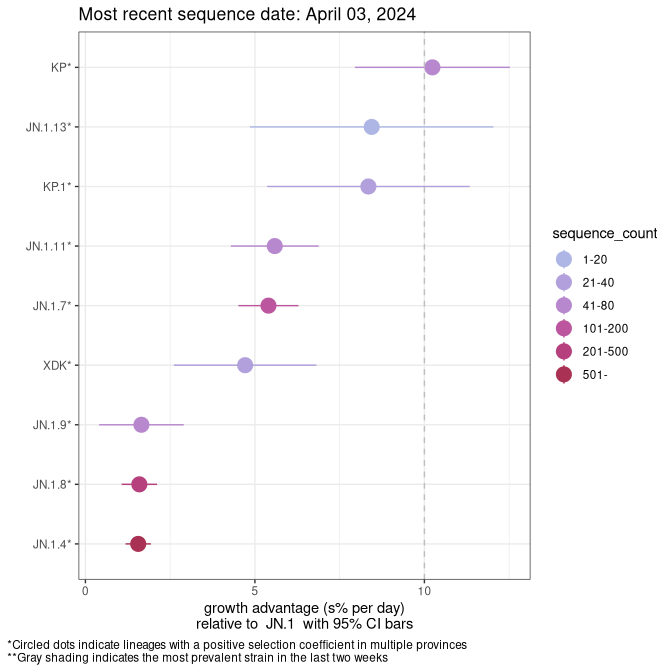
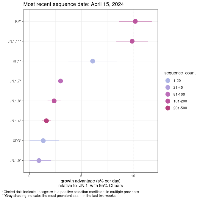
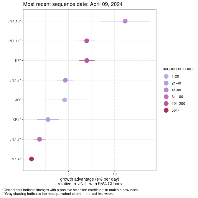
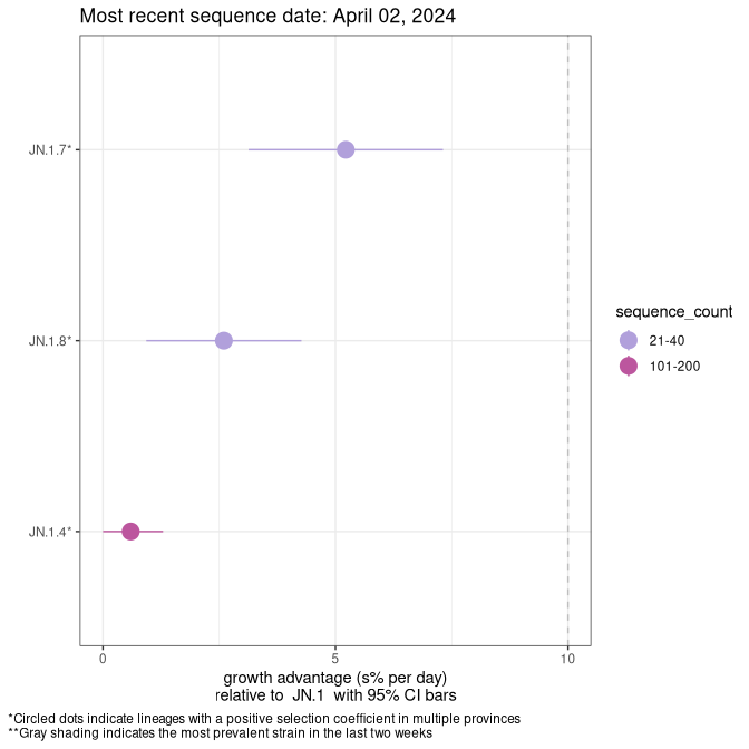
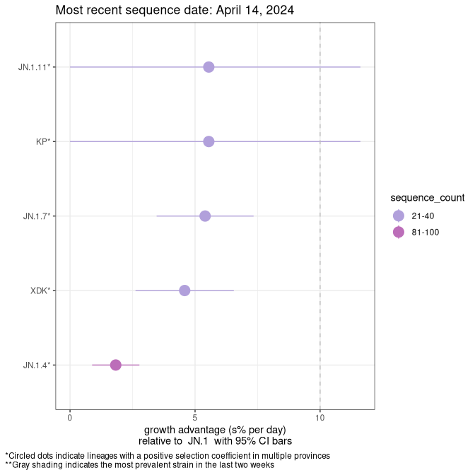
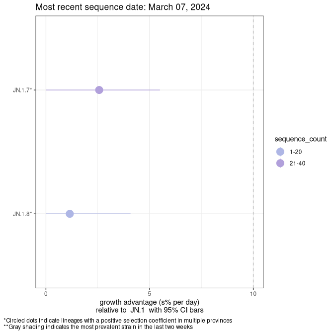
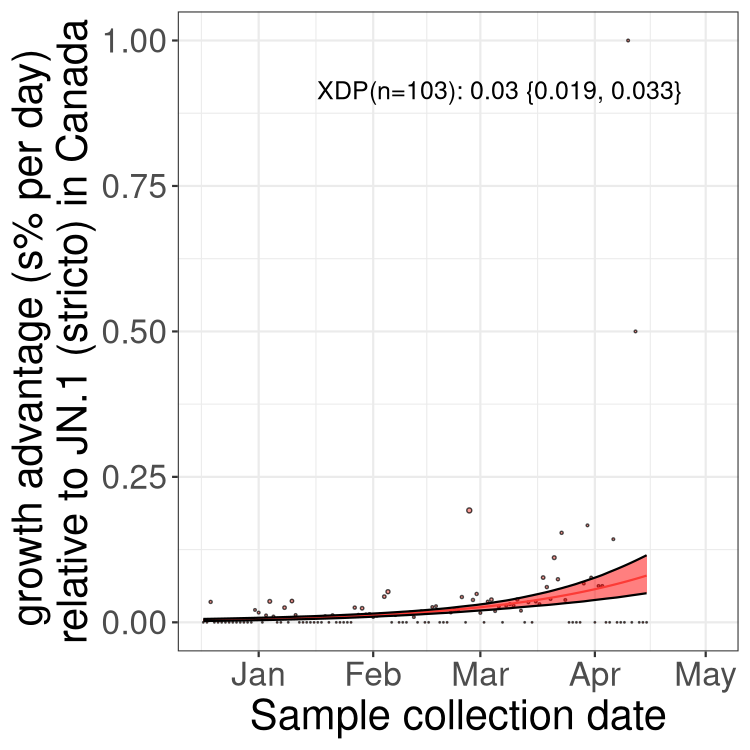
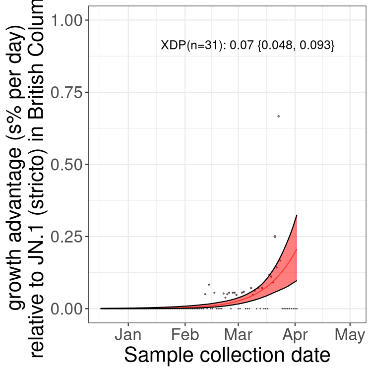
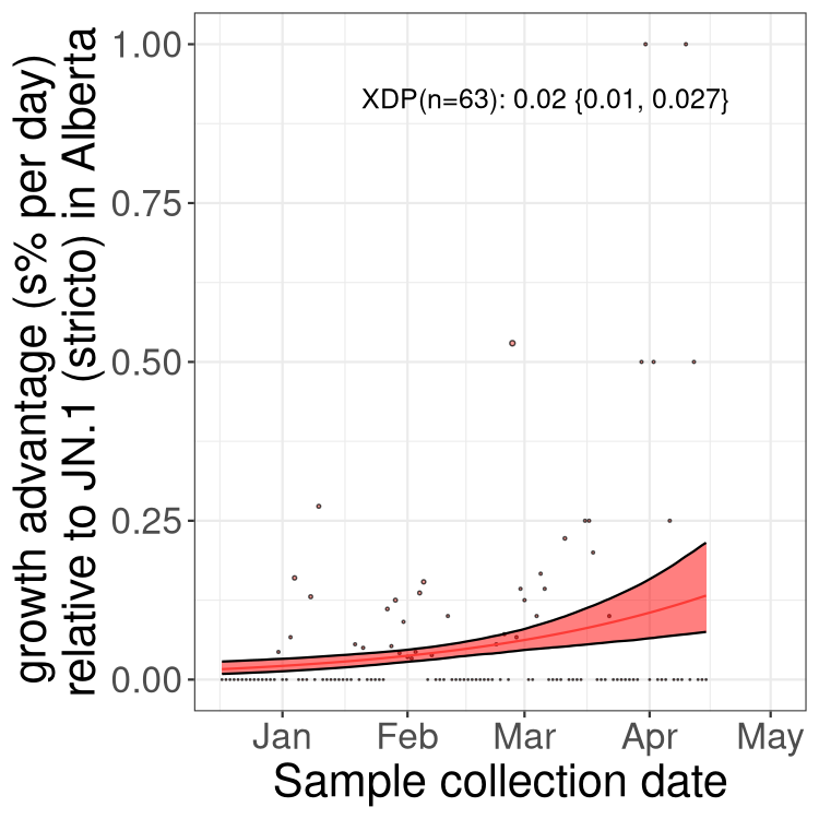
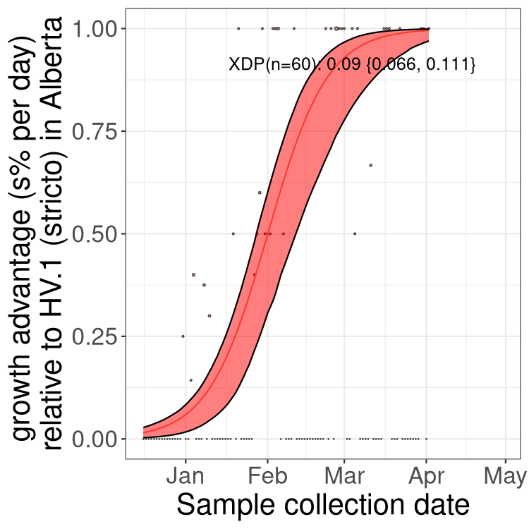
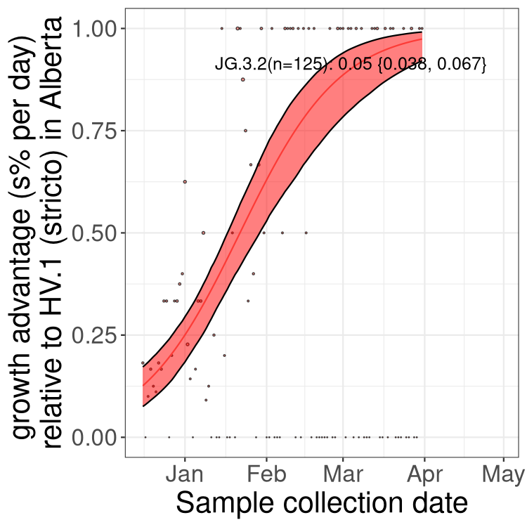
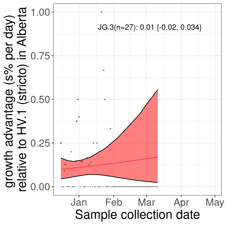
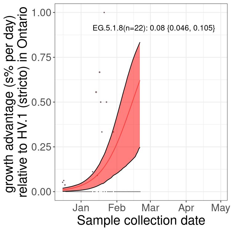
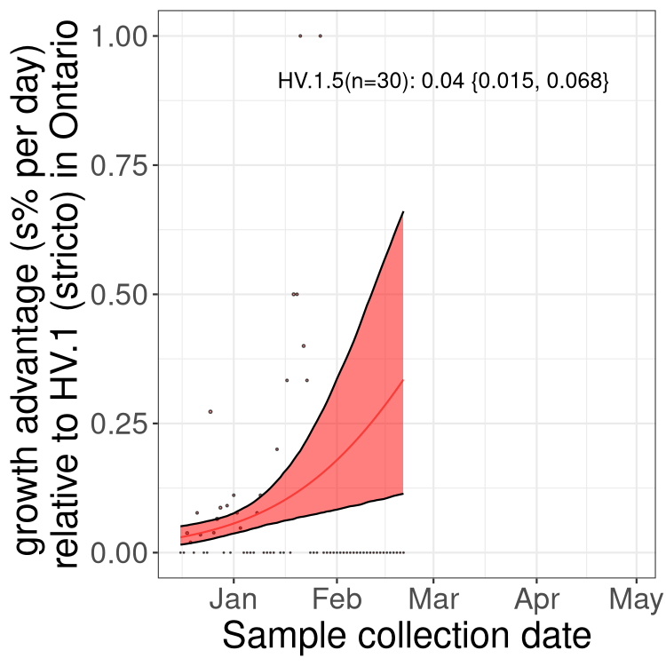
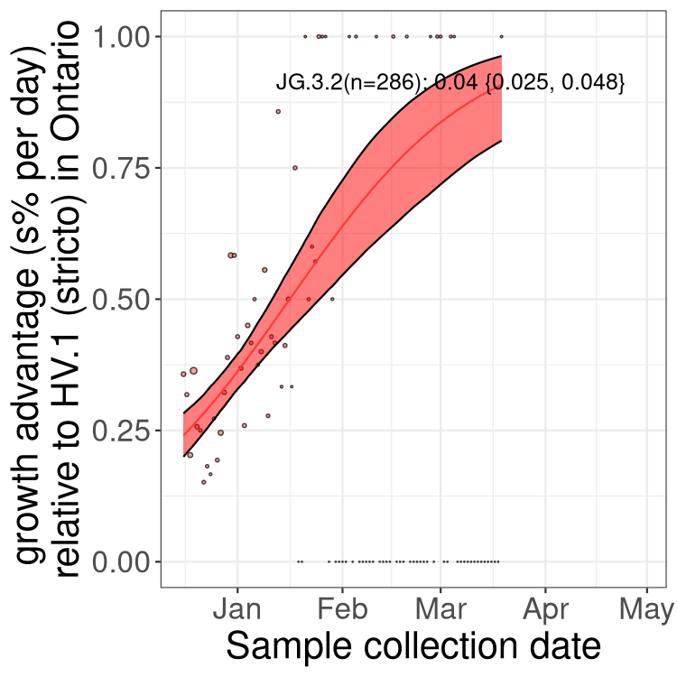
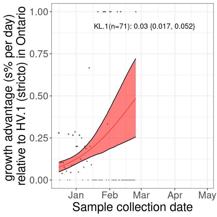
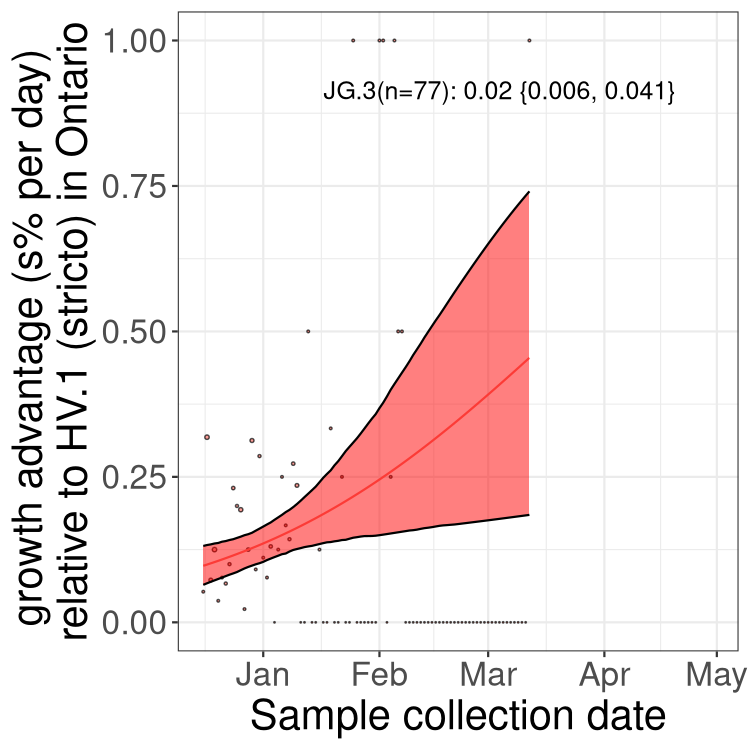
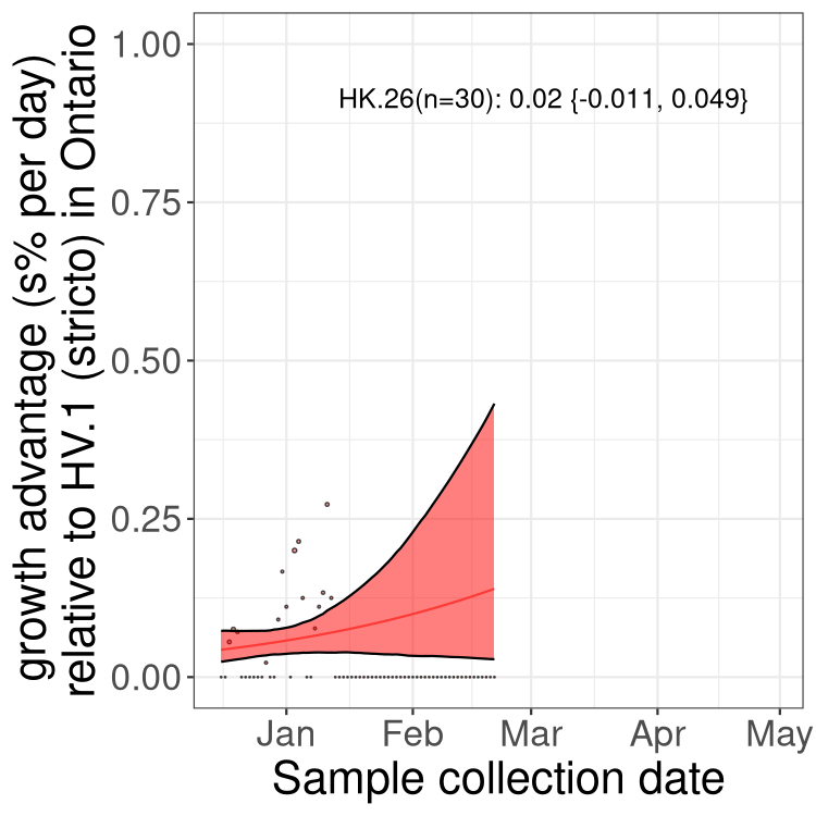
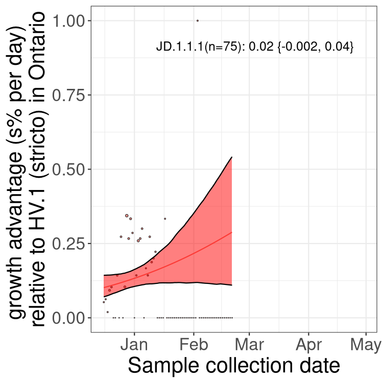
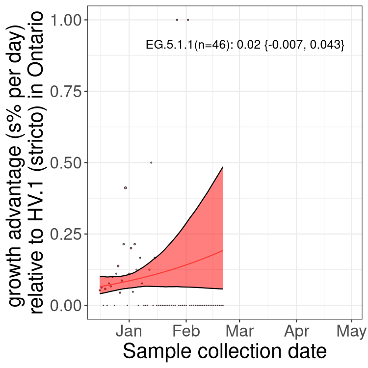
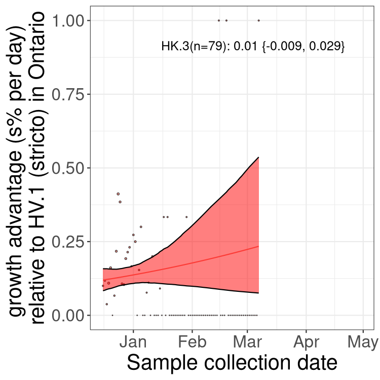
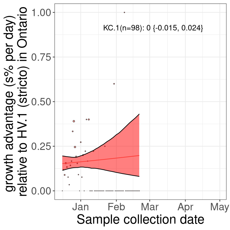
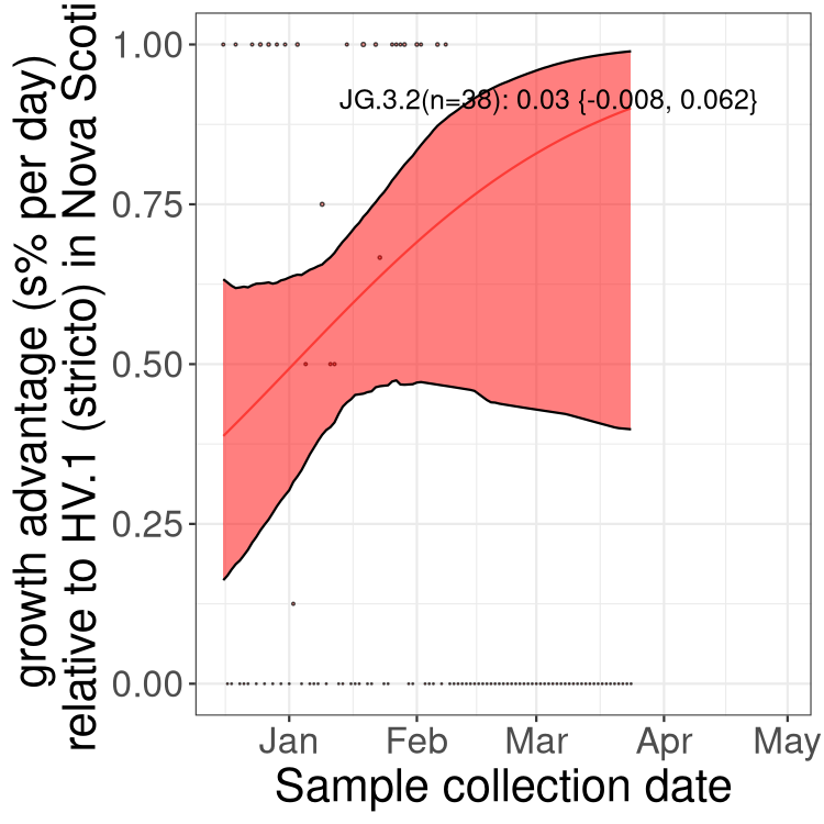
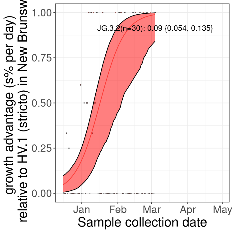
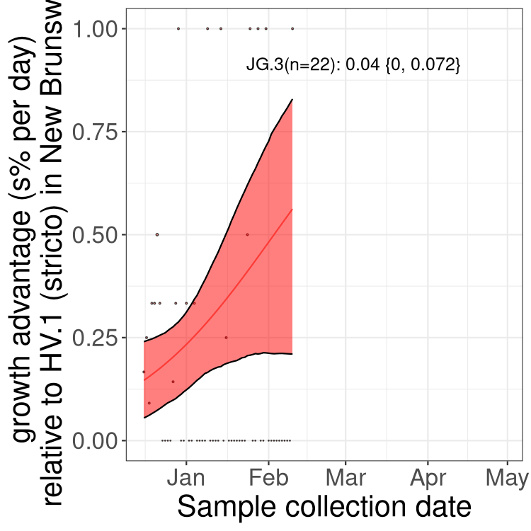
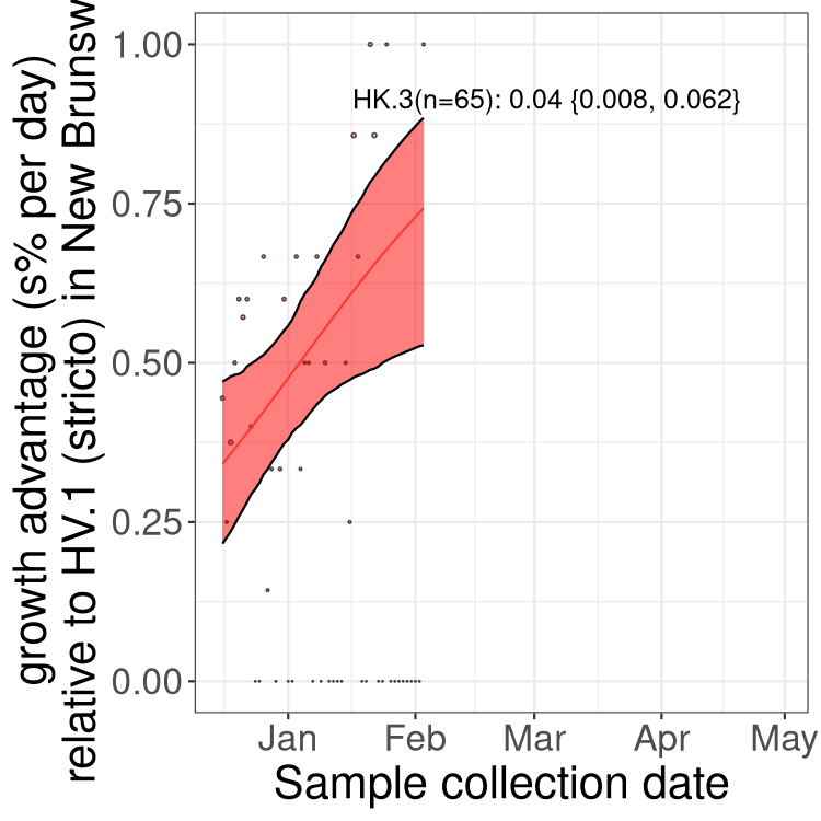
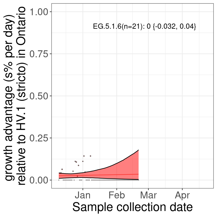
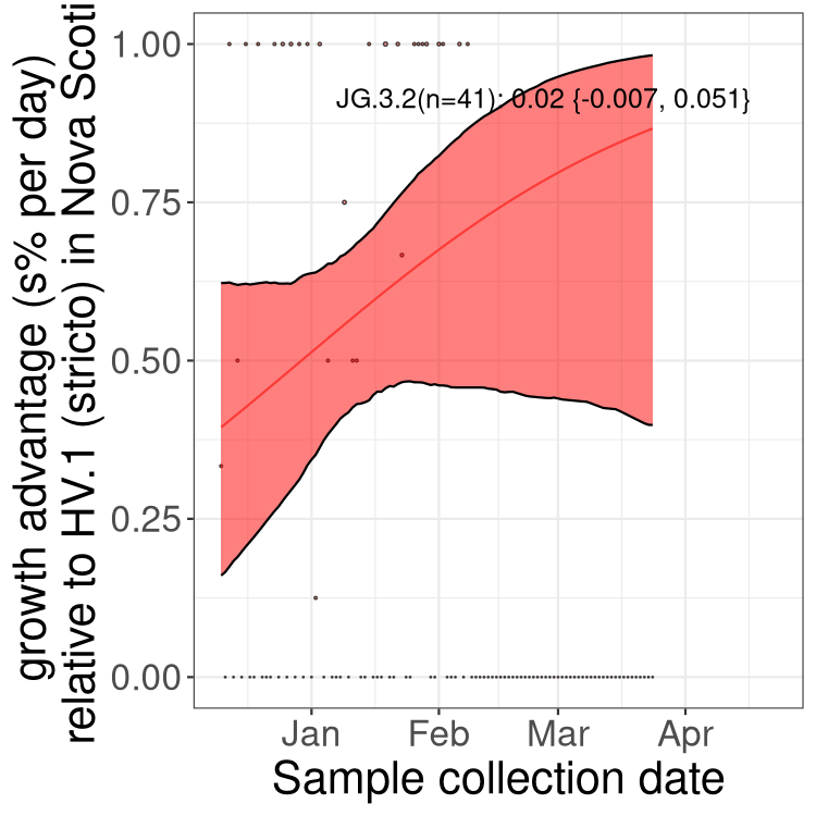
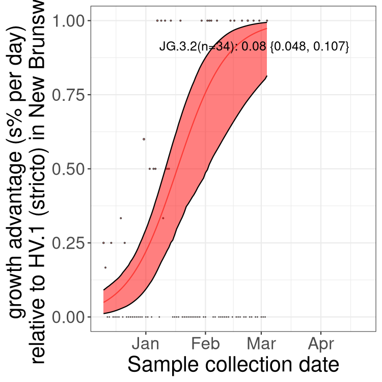
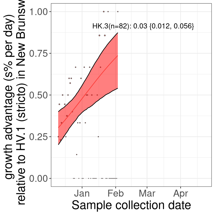
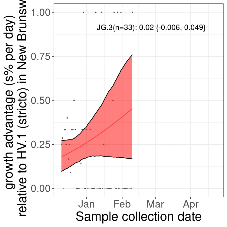
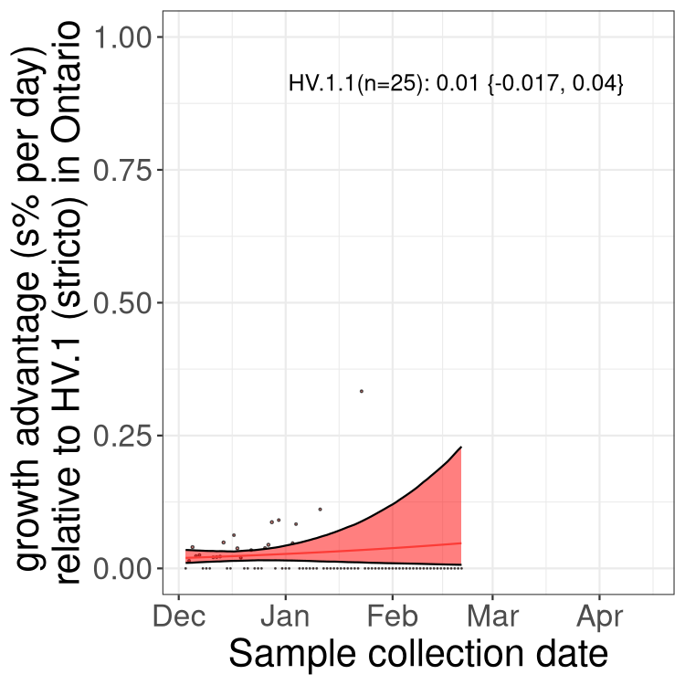
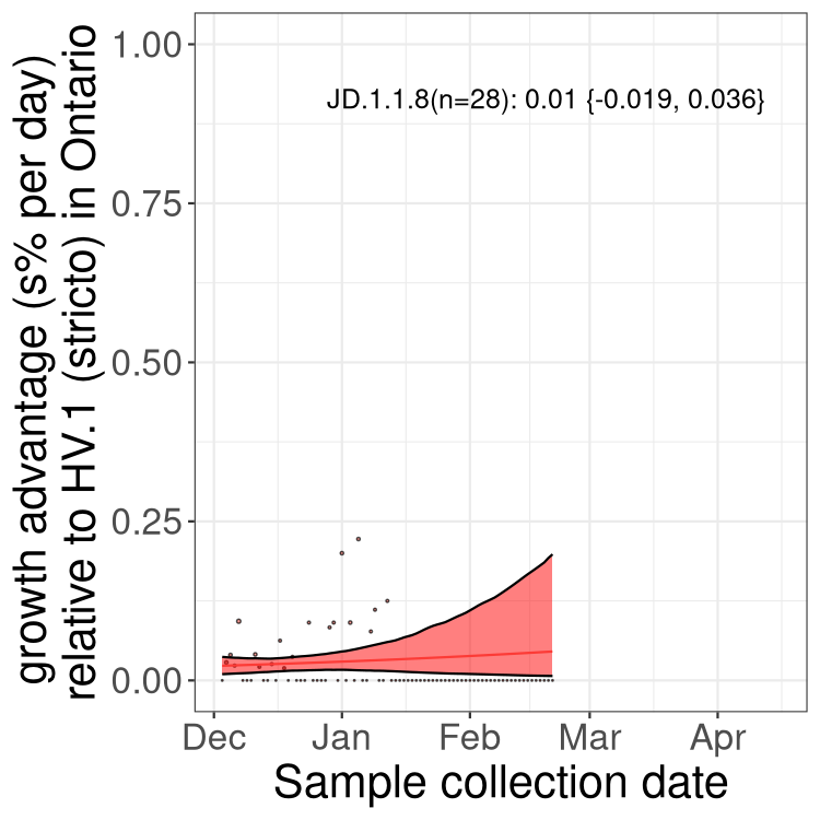
Fastest growing lineages
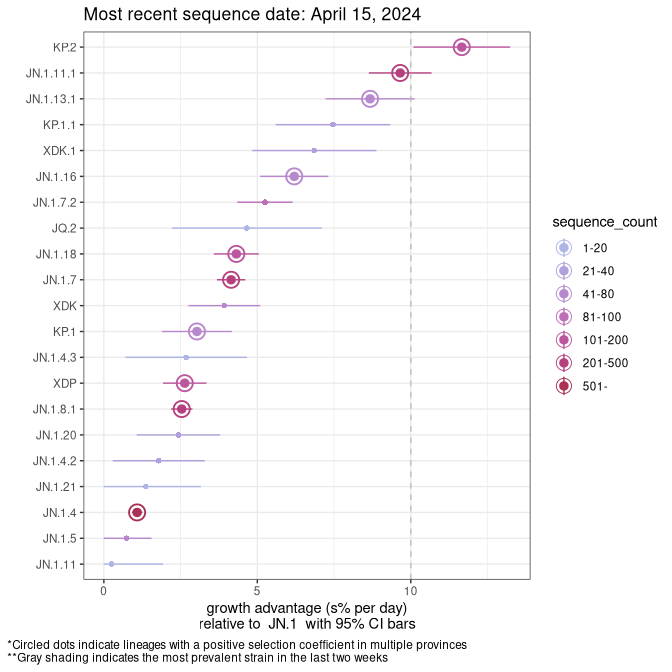
Here we show the selection estimates and their 95% confidence intervals for SARS-CoV-2 lineages with more than 10 sequences in present in a region since 2025-12-10, and with enough data to estimate the confidence interval. Each selection estimate measures the growth rate relative to XFG.3 stricto (i.e., sequences designated as XFG.3 and not its descendants). Plots showing the change in variant frequency over time in Canada as a whole are given below for lineages with more than 50 sequences. For Canada-wide plot, a dot with a circle border indicates lineages with a positive selection coefficient in multiple provinces. The most prevelant lineage in the last two weeks is highlighted in grey. A table of the selection estimates is available for download below.
Growth advantage of 0-5% corresponds to doubling times of more than two weeks, with 5-10% reflecting one to two week doubling times and over 10% representing significant growth of less than one week doubling time. Note that estimating selection of sub-variants with low sequence counts (points with less than 100 counts) is prone to error, such as mistaking one-time super spreader events or pulses of sequence data from one region as selection. Estimates with lower sequence counts in one region should be considered as very preliminary.
Plot (stricto)
This plot highlights single lineages that are growing fastest.
Canada
Plot single lineages in Canada *
BC
Plot single lineages in British Columbia
AB
Plot single lineages in Alberta
SK
Plot single lineages in Saskatchawan
MB
Plot single lineages in Manitoba

ON
Plot single lineages in Ontario
QC
Plot single lineages in Quebec
NS
Plot single lineages in Nova Scotia
NB
Plot single lineages in New Brunswick
NL
Plot single lineages in Newfoundland and Labrador
Plot (non stricto)
This plot highlights the groups of related lineages that are growing fastest (e.g., JN.1* is the monophyletic clade that includes JN.1.7 and all other JN.1 sublineages, excluding recombinants.
Canada
Plot single lineages in Canada
BC
Plot single lineages in British Columbia
AB
Plot single lineages in Alberta
SK
Plot single lineages in Saskatchawan

MB
Plot single lineages in Manitoba

ON
Plot single lineages in Ontario
QC
Plot single lineages in Quebec
NS
Plot single lineages in Nova Scotia
NB
Plot single lineages in New Brunswick
NL
Plot single lineages in Newfoundland and Labrador
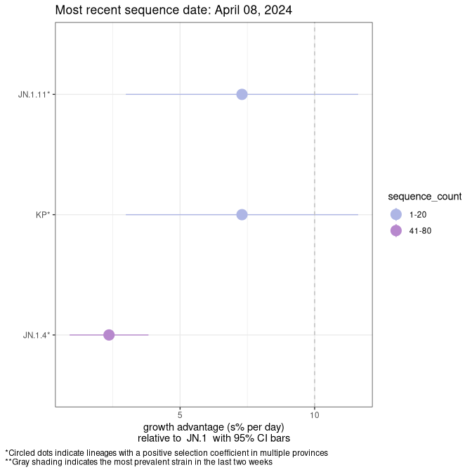
Table of all the selection estimates
Sublineages selection
BA.2 sublineages
Here we show the trends of the various BA.2.* sublineages over time, excluding any recombinants, relative to the frequency of XFG.3 by itself (shown for sublineages with at least 50 (Canada) or 20 (provinces) cases). Proportions shown here are only among XFG.3 (stricto) and the lineage illustrated. Note that these plots are not necessarily representative of trends in each province and that mixing of data from different provinces may lead to shifts in frequency that are not due to selection.
Canada
Canada
Only the three most strongly selected variants are displayed. Click
here to see the rest.


BC
British Columbia
AB
Alberta
SK
Saskatchawan
MB
Manitoba
ON
Ontario
Only the three most strongly selected variants are displayed. Click
here to see the rest.


QC
Quebec
NS
Nova Scotia

NB
New Brunswick
NL
Newfoundland and Labrador
NULL
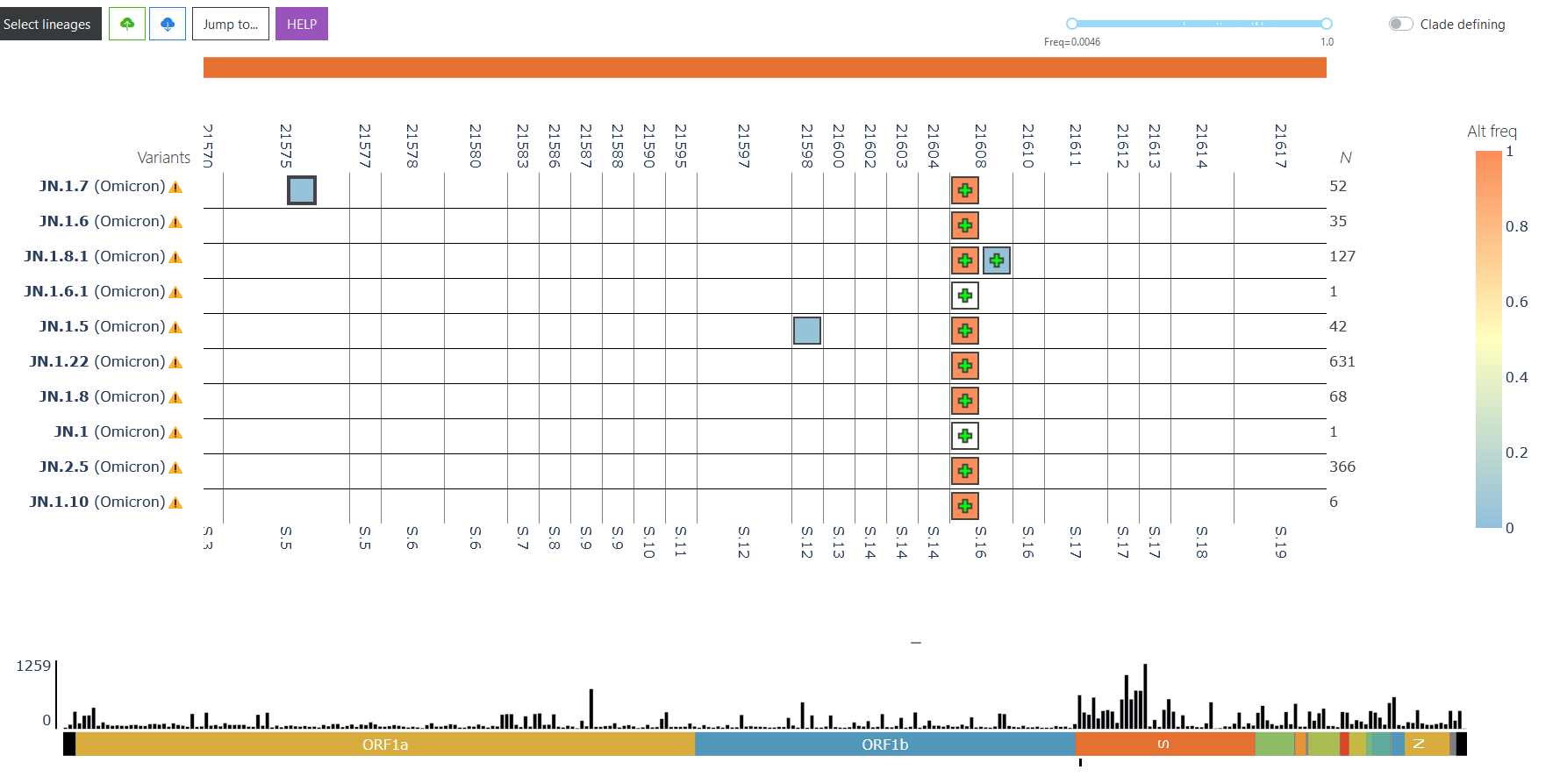
VIRUS-MVP: Mutational composition of Omicron
The image below is a screenshot from VIRUS-MVP showing a snapshot of the mutations from lineages actively circulating in Canada. Please click on the link to scan the entire genome and examine the functional impact of the mutations. More details, click on the image below or see https://virusmvp.org/covid-mvp.
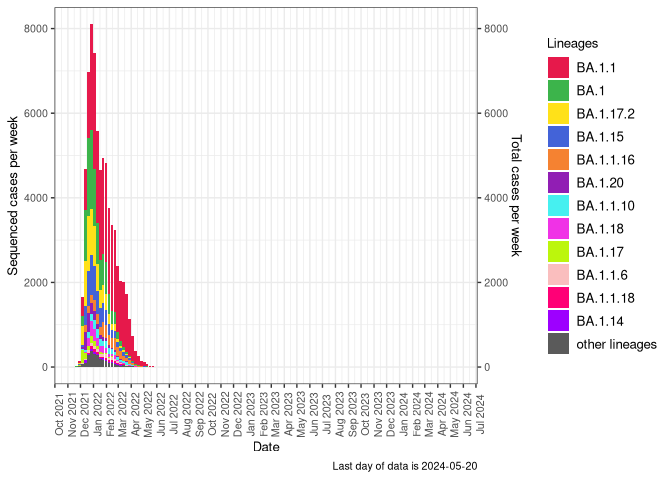
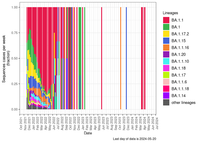
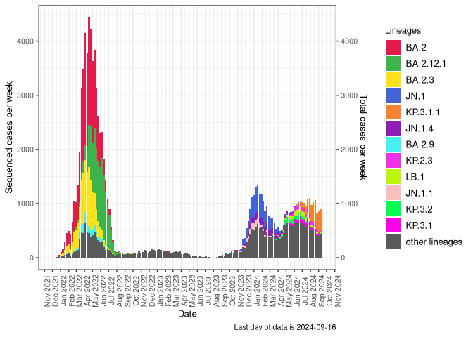
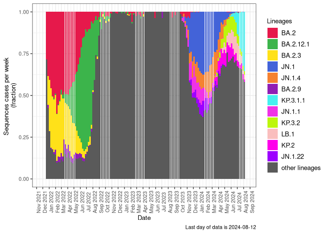
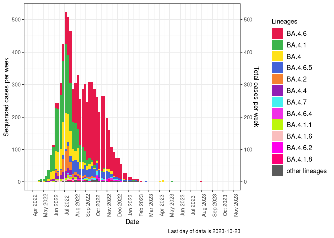
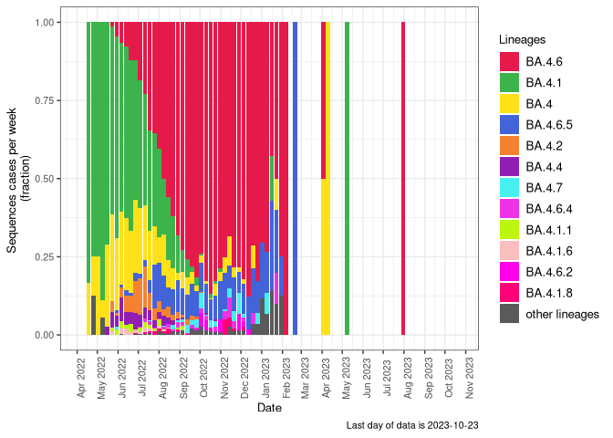
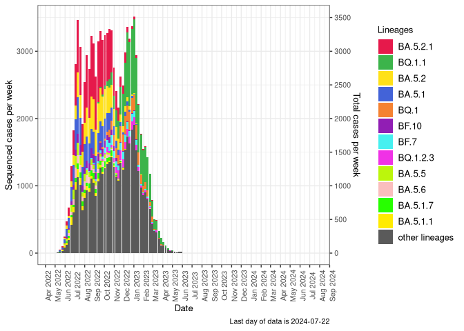
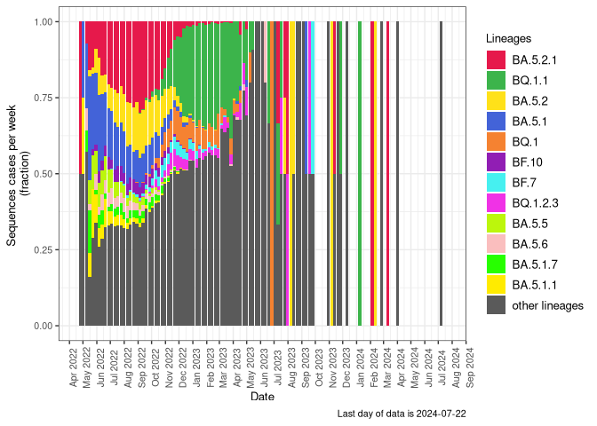
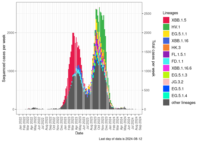
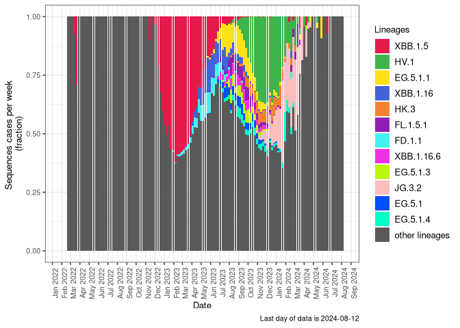
Variants in Canada over time
This plot shows the changing composition of sequences for all Canadian data posted to the VirusSeq Portal according to Pango lineage designation, up to 19 April, 2026. Because sampling and sequencing procedures vary by region and time, this does not necessarily reflect the true composition of SARS-CoV-2 viruses in Canada over time.
Canadian trees
Below is an interactive visualization of a subsampled phylogenetic snapshot of SARS-CoV-2 genomes from Canada. Please see methods for details.
The x-axis of the time tree represents the estimated number of years from today for which the root emerged. The x-axis of the diversity trees shows the number of mutations from the outgroup.
Hovering over a node will display a tool tip with sequence metadata, clicking on a node with the tooltip shown will copy the isolate ID to your clipboard.
### metadata and trees
source("scripts/tree.r")
# load trees from files
mltree <- read.tree(paste0(params$datadir,"/aligned_nonrecombinant_sample1.rtt.nwk"))
ttree <- read.tree(paste0(params$datadir,"/aligned_nonrecombinant_sample1.timetree.nwk"))
recombTTree <- read.tree(paste0(params$datadir,"/aligned_recombinant_X_sample1.timetree.nwk"))
recombMLree <- read.tree(paste0(params$datadir,"/aligned_recombinant_X_sample1.rtt.nwk"))
#stopifnot(all(sort(mltree$tip.label) == sort(ttree$tip.label)))
dateseq <- seq(ymd('2019-12-01'), ymd('2022-12-01'), by='3 month')
# tips are labeled with [fasta name]_[lineage]_[coldate]
# extracting just the first part makes it easier to link to metadata
mltree$tip.label <- reduce.tipnames(mltree$tip.label)
ttree$tip.label <- reduce.tipnames(ttree$tip.label)
recombTTree$tip.label <- reduce.tipnames(recombTTree$tip.label)
fieldnames<- c("fasta_header_name", "province", "host_gender", "host_age_bin",
"sample_collected_by", "purpose_of_sampling",
"lineage", "pango_group","week", "GID")
# extract rows from metadata table that correspond to ttree
metasub1 <- meta[meta$fasta_header_name%in% ttree$tip.label, fieldnames]
# sort rows to match tip labels in tree
metasub1 <- metasub1[match(ttree$tip.label, metasub1$fasta_header_name), ]
#omi tree metadata
#metasub_omi <- metasub1[grepl("Omicron",metasub1$pango_group ), ]
#recomb tree metadata
mmetasub_recomb <- meta[meta$fasta_header_name%in% recombTTree$tip.label, fieldnames]
mmetasub_recomb <- mmetasub_recomb[match(recombTTree$tip.label, mmetasub_recomb$fasta_header_name), ]
#scale to number of mutations
mltree$edge.length <- mltree$edge.length*29903
mltree <- ladderize(mltree, FALSE)
recombMLree$edge.length <- recombMLree$edge.length*29903
recombMLree <- ladderize(recombMLree, FALSE)
#enforce a non zero branch length so lines can be drawn in javascript
###Time Tree
ttree$edge.length[ttree$edge.length == 0] <- 1e-4
#ttree <- ladderize(ttree, FALSE)
recombTTree$edge.length[recombTTree$edge.length == 0] <- 1e-4
#recombTTree <- ladderize(recombTTree, FALSE)
hab=unique(meta$host_age_bin)
hab=hab[order(hab)]
months=unique(meta$month)
months=as.character(months[order(months)])
weeks=unique(meta$week)
weeks=as.character(weeks[order(weeks)])
presetColors=data.frame(name=c("other",
VOCVOI$name,
hab,
months,
weeks),
color=c("#777777",
VOCVOI$color,
rev(hcl.colors(length(hab)-1, "Berlin")),"#777777",
hcl.colors(length(months), "Berlin"),
hcl.colors(length(weeks), "Berlin")
))
#suppressWarnings({
# res <- ace(metasub1$pango.group, ttree2, type="discrete", model="ER")
#})
#idx <- apply(res$lik.anc, 1, which.max)[2:nrow(res$lik.anc)] # exclude root edge
#anc <- levels(as.factor(metasub1$pango.group))[idx]
source("scripts/tree.r")
timeTreeJsonObj <- DrawTree(ttree, metasub1, "timetree", presetColors, fieldnames=fieldnames)
recombTimeTreeJsonObj <- DrawTree(recombTTree, mmetasub_recomb, "recombtimetree", presetColors, "lineage", fieldnames= fieldnames)
#diversity ML tree
diversityTreeJsonObj <- DrawTree(mltree, metasub1, "mltree", presetColors, fieldnames=fieldnames)
recombDiversityTreeJsonObj <- DrawTree(recombMLree, mmetasub_recomb, "recombmltree", presetColors, "lineage", fieldnames=fieldnames)
#write(recombDiversityTreeJsonObj, "downloads/test.json")
### omicron diversity tree
#MLtree_omi<-keep.tip(mltree, metasub_omi$fasta_header_name)
#OmicrondiversityTreeJsonObj <- DrawTree(MLtree_omi, metasub_omi, "omimltree", presetColors, fieldnames=fieldnames)