
CAMEO - Duotang
CAMEO - Duotang
Duotang, a genomic epidemiology analyses and mathematical modelling notebook
Pillar 6 - CAMEO, CoVaRR-Net
23 June, 2023
Survey request
Doutang, VirusSeq Data portal, and Viral AI would like to improve your user experience. Please take a few minutes to respond to this survey.
SARS-CoV-2 In Canada
Introduction
This notebook was built to explore Canadian SARS-CoV-2 genomic and epidemiological data with the aim of investigating viral evolution and spread. It is developed by the CAMEO team (Computational Analysis, Modelling and Evolutionary Outcomes Group) associated with the Coronavirus Variants Rapid Response Network (CoVaRR-Net) for sharing with collaborators, including public health labs. These analyses are freely available and open source, enabling code reuse by public health authorities and other researchers for their own use.
Canadian genomic and epidemiological data will be regularly pulled from various public sources (see list below) to keep these analyses up-to-date. Only representations of aggregate data will be posted here.
Important limitations
These analyses represent only a snapshot of SARS-CoV-2 evolution in Canada. Only some infections are detected by PCR testing, only some of those are sent for whole-genome sequencing, and not all sequences are posted to public facing reposittories. Sequencing volumes and priorities have changed during the pandemic, and the sequencing strategy is typically a combination of prioritizing outbreaks, travellers, public health investigations, and random sampling for genomic surveillance.
For example, specific variants or populations might be preferentially sequenced at certain times in certain jurisdictions. When possible, these differences in sampling strategies are mentioned but they are not always known. With the arrival of the Omicron wave, many jurisdictions across Canada reached testing and sequencing capacity mid-late December 2021 and thus switched to targeted testing of priority groups (e.g., hospitalized patients, health care workers, and people in high-risk settings). Therefore, from this time onward, case counts are likely underestimated and the sequenced virus diversity is not necessarily representative of the virus circulating in the overall population.
Thus, interpretation of these plots and comparisons between health regions should be made with caution, considering that the data may not be fully representative. These analyses are subject to frequent change given new data and updated lineage designations.
The last sample collection date is 05 June, 2023
Current situation
XBB.1.5 “stricto” is decreasing now, with XBB.1.5 with S:456L and other variants with this mutation growing, plus also XBB.1.16 which has both spike and non-spike mutations proposed to be advantageous. Different variants are predominating in some different provinces depending on timing of their introduction (for example, FD.1.1 was introduced earlier in Quebec). Some XBB.1.9, and XBB.2.3 variants are still growing, however XBB.1.16 variants are outcompeting these in most regions. All of these variants have mutations that would confer additional immune evasion and/or infectivity. Any saltation variants (variants with sudden, large mutational changes) are being closely tracked.
Variants of current interest, due to their current/potential growth advantage, mutations of potential functional significance, or spread in other countries:
- FD.1.1 (subvariant of XBB.1.5.15 with S:F456L)
- FE.1 (subvariant of XBB.1.18.1 with S:456L)
- Multiple XBB.1.5 subvariants including those that have S:F456L
- XBB.1.16 which has S:T478R (with a particular interest in those with S:F456L)
- XBB.1.9.1, XBB.1.9.2, FL.5 (which have non-spike mutations of note, with a particular interest in those with S:Q613H OR with S:F456L plus NS6:Y49H - aka orf6:y49h)
- XBB.2.3, XBB.2.3.2, XBB.2.3.3 (has mutation S:P521S, with an interest in those also with mutation 478R)
…plus any saltation variants and sublineages with additional combinations of the mutations below.
Mutations of interest include:
- S:F456L (evidence of increased immune evasion versus recent variants and a mutation growing in prevalence in multiple lineages in multiple regions)
- S:T478R (aka S:K478R - the S:T478K mutation occurred first). Evidence of increased infectivity when introduced into XBB.1.5. Associated with XBB.1.16 (which has additional mutations like S:E180V that may counteract this mutations advantage) but now seen in additional variants like XBB.2.3.
- S:P521S (evidence it could increase human ACE2 receptor binding/infectivity - associated with XBB.2.3 variants)
- S:Q613H (growing and seen in XBB.1.5, CH.1.1 and XBB.1.9.1)
- ORF1b:D1746Y (aka NSP14_D222Y - in XBB.1.16 variants)
- ORF9b:I5T (note its a synonymous mutation in the overlapping N gene)
- ORF9b:N55S (synonymous mutation in N)
Plus other mutations identified through deep mutation scanning and the SARS-CoV-2 RBD antibody escape calculator. See:
- https://jbloomlab.github.io/SARS2-RBD-escape-calc/
- Greaney, Starr, & Bloom, Virus Evolution, 8:veac021 (2022)
- Cao et al, Nature, 614:521-529 (2023)
- Yisimayi et al, bioRxiv, DOI 10.1101/2023.05.01.538516 (2023)
Omicron sublineages in Canada
Here we take a look, sub-dividing the major sub-lineages currently circulating in Canada. (Click and drag to zoom, double click to reset. Clicking on an item in the legend will hide it, double clicking an item in legend will hide everything else but that item.)
Last 120 days
Last 120 days sublineages starting from 2023-02-05 (Frequency Table Download)
BA.1
BA.1 sublineages (Frequency Table Download)
BA.2
BA.2 sublineages (Frequency Table Download)
BA.4
BA.4 sublineages (Frequency Table Download)
BA.5
BA.5 sublineages (Frequency Table Download)
Recombinants
Recombinants sublineages (Frequency Table Download)
Selection on Omicron
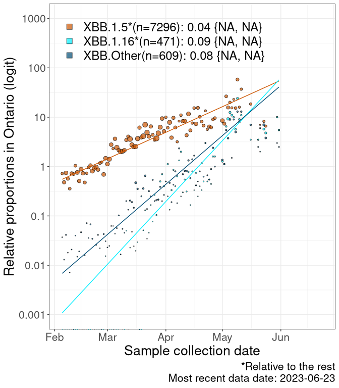
Here we examine the relative rate of spread of the different sublineages of Omicron currently in Canada. Specifically, we determine if a new or emerging lineage has a selective advantage (s), and by how much, against a reference lineage previously common in Canada (see the methods for more details about selection and how it is estimated).
Currently, the major group of Omicron lineages rising in frequency are the XBB.* group, dominated by the XBB.1.5* lineages which is near it’s peak. There are also several other XBB lineages showing a selective advantage. The previous dominant lineage, BQ.*, is nearly at the bottom, however several of it’s descendant are beginning to grow again. See Fastest Growing Lineages for details on lineages showing positive selection.
We first show this growth of XBB.1.5*, XBB.1.16*, or XBB.Other, relative to the remaining strains, which consist predominantly of BQ.*. Left plot: y-axis is the proportion of sub-lineages XBB.1.5*, XBB.1.16*, and XBB.Other relative to the remaining strains; right plot: y-axis describes the logit function, log(freq(XBB.1.5*, XBB.1.16*, or XBB.Other)/freq(the rest)), which gives a straight line whose slope is the selection coefficient if selection is constant over time (see methods).
For comparison, Alpha had a selective advantage of s ~ 6%-11% per day over preexisting SARS-CoV-2 lineages, and Delta had a selective advantage of about 10% per day over Alpha.
Caveat: These selection analyses must be interpreted with caution due to the potential for non-representative sampling, lags in reporting, and spatial heterogeneity in prevalence of different sublineages across Canada. Provinces that do not have at least 20 sequences of a lineage during this time frame are not displayed.
Canada
Canada


BC
British Columbia


AB
Alberta


SK
Saskatchawan


MB
Manitoba


ON
Ontario

QC
Quebec


NS
Nova Scotia


NB
New Brunswick


NL
Newfoundland and Labrador


NULL
Case count trends by variant
These plots follow reported cases per 100,000 individuals (green dots), ignoring the most recent case counts (hollow circles), which are generally underestimated as data continues to be gathered. A cubic spline is fit to the log of these case counts to illustrate trends (top curve). The last two days of accurate case counts are then used to estimate the daily exponential growth rate \(r\) in COVID-19 cases. The fit from the “Selection on Omicron” section above is used to show how each of the sub-lineages is growing or shrinking, with the corresponding growth rate \(r\) for each sub-lineage on the last two days of accurate case counts. For detailed methodology, please see the methods section in the appendix.
Canada
Canada

BC
British Columbia

AB
Alberta

SK
Saskatchawan

MB
Manitoba

ON
Ontario

QC
Quebec

NS
Nova Scotia

NB
New Brunswick

NL
Newfoundland and Labrador

NULL
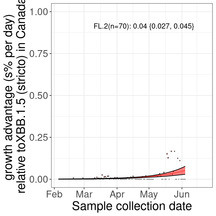
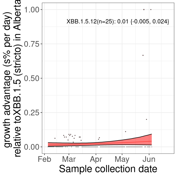
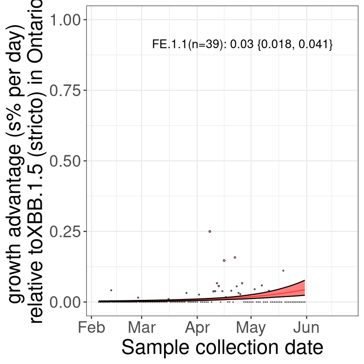
Fastest growing lineages
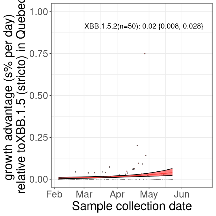
Here we show the selection estimates and their 95% confidence intervals for Pango lineages with more than 10 sequences in Canada since 2023-02-05 and with enough data to estimate the confidence interval. Each selection estimate measures the growth rate relative to XBB.1.5 stricto (i.e., sequences designated as XBB.1.5 and not its descendants, like XBB.1.5.1). Plots showing the change in variant frequency over time in Canada are given below for lineages with more than 50 sequences.
Plot (stricto)
Growth advantage of 0-5% corresponds to doubling times of more than two weeks, with 5-10% reflecting one to two week doubling times and over 10% representing significant growth of less than one week doubling time. Note that estimating selection of sub-variants with low sequence counts (less than 100 dots) is prone to error, such as mistaking one-time super spreader events or pulses of sequence data from one region as selection. Estimates with lower sequence counts in one region should be considered as very preliminary. For Canada-wide plot, a dot with a circle border indicates lineages with a positive selection coefficient in multiple provinces.
Canada
Plot single lineages in Canada *

BC
Plot single lineages in British Columbia

AB
Plot single lineages in Alberta

SK
Plot single lineages in Saskatchawan

MB
Plot single lineages in Manitoba

ON
Plot single lineages in Ontario

QC
Plot single lineages in Quebec

NS
Plot single lineages in Nova Scotia

NB
Plot single lineages in New Brunswick

NL
Plot single lineages in Newfoundland and Labrador

Plot (non stricto)
This plot highlights the groups of related lineages that are growing fastest (e.g., BQ.1* is the monophyletic clade that includes BQ.1.1 and all other BQ.1 sublineages.
Again, Growth advantage of 0-5% corresponds to doubling times of more than two weeks, with 5-10% reflecting one to two week doubling times and over 10% representing significant growth of less than one week doubling time. Note that estimating selection of sub-variants with low sequence counts (less than 100 dots) is prone to error, such as mistaking one-time super spreader events or pulses of sequence data from one region as selection. Estimates with lower sequence counts in one region should be considered as very preliminary. For Canada-wide plot, a dot with a circle border indicates lineages with a positive selection coefficient in multiple provinces.
Canada
Plot single lineages in Canada

BC
Plot single lineages in British Columbia

AB
Plot single lineages in Alberta

SK
Plot single lineages in Saskatchawan

MB
Plot single lineages in Manitoba

ON
Plot single lineages in Ontario

QC
Plot single lineages in Quebec

NS
Plot single lineages in Nova Scotia

NB
Plot single lineages in New Brunswick

NL
Plot single lineages in Newfoundland and Labrador

Table of all the selection estimates
Sublineages selection
BA.2 and XBB sublineages
Here we show the trends of the various BA.2.* sublineages over time, relative to the frequency of XBB.1.5 by itself (shown for sublineages with at least 50 (Canada) or 20 (provinces) cases). Proportions shown here are only among XBB.1.5 (stricto) and the lineage illustrated. Note that these plots are not necessarily representative of trends in each province and that mixing of data from different provinces may lead to shifts in frequency that are not due to selection.
Canada
Canada


Only the three most strongly selected variants are displayed. Click here to see the rest.


BC
British Columbia


Only the three most strongly selected variants are displayed. Click here to see the rest.


AB
Alberta


Only the three most strongly selected variants are displayed. Click here to see the rest.


SK
Saskatchawan

MB
Manitoba

ON
Ontario


Only the three most strongly selected variants are displayed. Click here to see the rest.


QC
Quebec


Only the three most strongly selected variants are displayed. Click here to see the rest.


NS
Nova Scotia

NB
New Brunswick

NL
Newfoundland and Labrador


NULL
BA.5 sublineages
Here we show the trends of the various BA.5* sublineages over time, relative to the frequency of XBB.1.5 by itself (shown for sublineages with at least 50 (Canada) or 20 (provinces) cases). Proportions shown here are only among XBB.1.5 (stricto) and the lineage illustrated. Note that these plots are not necessarily representative of trends in each province and that mixing of data from different provinces may lead to shifts in frequency that are not due to selection.
Canada
Canada

BC
British Columbia

AB
Alberta

SK
Saskatchawan

MB
Manitoba

ON
Ontario

QC
Quebec

NS
Nova Scotia

NB
New Brunswick

NL
Newfoundland and Labrador

NULL
Mutational composition of Omicron
Tabulation of the most predominant mutational changes in Omicron, with adjacent rows comparing the composition of Canadian sublineages to that sublineage globally.

Mutational profile of Omicron and its sublineages in Canada and globally for the most prevalent (>75%) point mutations in each category (based on the 499218 genomes available on VirusSeq on June 23, 2023).
Variants in Canada over time
This plot shows the changing composition of sequences for all Canadian data posted to the VirusSeq Portal according to Pango lineage designation (Pango version 4.2 (Viral AI)), up to 2023-06-10. Because sampling and sequencing procedures vary by region and time, this does not necessarily reflect the true composition of SARS-CoV-2 viruses in Canada over time.
Historical notes
From the beginning of the pandemic to the fall of 2021, Canadian sequences were mostly of the wildtype lineages (pre-VOCs). By the beginning of summer 2021, the VOCs Alpha and Gamma were the most sequenced lineages overall in Canada. The Delta wave grew during the summer of 2021 with sublineages AY.25 and AY.27 constituting sizeable proportions of this wave. Omicron arrived in November of 2021 and spread in three main waves, first BA.1* (early 2022), then BA.2* (spring 2022), then BA.5* (summer 2022). Current, multiple sublineages of Omicron persist, with emerging sublineages spreading, such as BQ.1.1 (a BA.5 sub-lineage).
There are two Pango lineages that have a Canadian origin and that predominately spread within Canada (with some exportations internationally): B.1.438.1 and B.1.1.176. Other lineages of historical interest in Canada:
- A.2.5.2 - an A lineage (clade 19B) that spread in Quebec, involved in several outbreaks before Delta arrived (see this post for more details: https://virological.org/t/recent-evolution-and-international-transmission-of-sars-cov-2-clade-19b-pango-a-lineages/711)
- B.1.2 - a USA lineage that spread well in Canada
- B.1.160 - an European lineages that spread well in Canada
This historical analysis is not being further updated, as we focus on more interactive data plots and the “Current situation” text above.
Canadian trees
Here we present a subsampled phylogenetic snapshot of SARS-CoV-2 genomes from Canada. The x-axis of the time tree represents the estimated number of years from today for which the root emerged. Due to the low number of XBB sequences, this estimate may not be accurate for the XBB* time tree. The x-axis of the diversity trees shows the number of mutations from the outgroup. Clicking on a node with the information tooltip shown will copy the isolate ID to your clipboard.
### metadata and trees
source("scripts/tree.r")
# load trees from files
mltree <- read.tree(paste0(params$datadir,"/aligned_nonrecombinant_sample1.rtt.nwk"))
ttree <- read.tree(paste0(params$datadir,"/aligned_nonrecombinant_sample1.timetree.nwk"))
recombTTree <- read.tree(paste0(params$datadir,"/aligned_recombinant_XBBS_sample1.timetree.nwk"))
recombMLree <- read.tree(paste0(params$datadir,"/aligned_recombinant_XBBS_sample1.rtt.nwk"))
#stopifnot(all(sort(mltree$tip.label) == sort(ttree$tip.label)))
dateseq <- seq(ymd('2019-12-01'), ymd('2022-12-01'), by='3 month')
# tips are labeled with [fasta name]_[lineage]_[coldate]
# extracting just the first part makes it easier to link to metadata
mltree$tip.label <- reduce.tipnames(mltree$tip.label)
ttree$tip.label <- reduce.tipnames(ttree$tip.label)
recombTTree$tip.label <- reduce.tipnames(recombTTree$tip.label)
fieldnames<- c("fasta_header_name", "province", "host_gender", "host_age_bin",
"sample_collected_by", "purpose_of_sampling",
"lineage", "pango_group","week", "GID")
# extract rows from metadata table that correspond to ttree
metasub1 <- meta[meta$fasta_header_name%in% ttree$tip.label, fieldnames]
# sort rows to match tip labels in tree
metasub1 <- metasub1[match(ttree$tip.label, metasub1$fasta_header_name), ]
#omi tree metadata
#metasub_omi <- metasub1[grepl("Omicron",metasub1$pango_group ), ]
#recomb tree metadata
mmetasub_recomb <- meta[meta$fasta_header_name%in% recombTTree$tip.label, fieldnames]
mmetasub_recomb <- mmetasub_recomb[match(recombTTree$tip.label, mmetasub_recomb$fasta_header_name), ]
#scale to number of mutations
mltree$edge.length <- mltree$edge.length*29903
mltree <- ladderize(mltree, FALSE)
recombMLree$edge.length <- recombMLree$edge.length*29903
recombMLree <- ladderize(recombMLree, FALSE)
#enforce a non zero branch length so lines can be drawn in javascript
###Time Tree
ttree$edge.length[ttree$edge.length == 0] <- 1e-4
#ttree <- ladderize(ttree, FALSE)
recombTTree$edge.length[recombTTree$edge.length == 0] <- 1e-4
#recombTTree <- ladderize(recombTTree, FALSE)
hab=unique(meta$host_age_bin)
hab=hab[order(hab)]
months=unique(meta$month)
months=as.character(months[order(months)])
weeks=unique(meta$week)
weeks=as.character(weeks[order(weeks)])
presetColors=data.frame(name=c("other",
VOCVOI$name,
hab,
months,
weeks),
color=c("#777777",
VOCVOI$color,
rev(hcl.colors(length(hab)-1, "Berlin")),"#777777",
hcl.colors(length(months), "Berlin"),
hcl.colors(length(weeks), "Berlin")
))
#suppressWarnings({
# res <- ace(metasub1$pango.group, ttree2, type="discrete", model="ER")
#})
#idx <- apply(res$lik.anc, 1, which.max)[2:nrow(res$lik.anc)] # exclude root edge
#anc <- levels(as.factor(metasub1$pango.group))[idx]
source("scripts/tree.r")
timeTreeJsonObj <- DrawTree(ttree, metasub1, "timetree", presetColors, fieldnames=fieldnames)
recombTimeTreeJsonObj <- DrawTree(recombTTree, mmetasub_recomb, "recombtimetree", presetColors, "lineage", fieldnames= fieldnames)
#diversity ML tree
diversityTreeJsonObj <- DrawTree(mltree, metasub1, "mltree", presetColors, fieldnames=fieldnames)
recombDiversityTreeJsonObj <- DrawTree(recombMLree, mmetasub_recomb, "recombmltree", presetColors, "lineage", fieldnames=fieldnames)
#write(recombDiversityTreeJsonObj, "downloads/test.json")
### omicron diversity tree
#MLtree_omi<-keep.tip(mltree, metasub_omi$fasta_header_name)
#OmicrondiversityTreeJsonObj <- DrawTree(MLtree_omi, metasub_omi, "omimltree", presetColors, fieldnames=fieldnames)Time Tree
XBB* time tree
Diversity Tree
XBB* Diversity tree
Root-to-tip analyses
The slope of root-to-tip plots over time provide an estimate of the substitution rate. A lineage with a steeper positive slope than average for SARS-CoV-2 is accumulating mutations at a faster pace, while a lineage that exhibits a jump up (a shift in intercept but not slope) has accumulated more than expected numbers of mutations in a transient period of time (similar to what we saw with Alpha when it first appeared in the UK).
Molecular clock estimates (based on three independent subsamples)
Here we show the estimate of the substitution rate for 3 independent subsamples of different variants of interest, with their 95% confidence interval.

Pango lineage table
Here we present a searchable table that provides a short description of each lineage as well information on the ancestor of that lineage.
Appendix
Future development
We are in the process of adding or would like to develop code for some of the following analyses:
- dN/dS (by variant and by gene/domains)
- Tajima’s D over time
- clustering analyses
- genomically inferred epidemiological parameters: R0, serial interval, etc.
With anonymized data on vaccination status, severity/outcome, reason for sequencing (e.g., outbreak, hospitalization, or general sampling), and setting (workplace, school, daycare, LTC, health institution, other), we could analyze genomic characteristics of the virus relative to the epidemiological and immunological conditions in which it is spreading and evolving. Studies on mutational correlations to superspreading events, vaccination status, or comparisons between variants would allow us to better understand transmission and evolution in these environments.
Methodology
Genome data and metadata are sourced from the Canadian VirusSeq Data Portal. Pango lineage assignments are generated using the pangoLEARN algorithm. Source code for generating this RMarkdown notebook can be found in [https://github.com/CoVaRR-NET/duotang].
Trees
Phylogenetic trees
Canadian genomes were obtained from the VirusSeq data on the June 23, 2023 and down-sampled to two genomes per lineage, province and month before October 2021, and five genomes per lineage, province and month after October 2021 (about 10,000 genomes in total). We used a Python wrapper of minimap2 (version 2.17) to generate multiple sequence alignments for these genome samples. A maximum likelihood (ML) tree was reconstructed from each alignment using the COVID-19 release of IQ-TREE (version 2.2.0). Outliers were identified in by root-to-tip regression using the R package ape and removed from the dataset. TreeTime was used to reconstruct a time-scaled tree under a strict molecular clock model. The resulting trees were converted into interactive plots with ggfree and r2d3.
Mutational composition
Mutation composition graph
We extracted mutation frequencies from unaligned genomes using a custom Python wrapper of minimap2 (version 2.17). These data were supplemented with genomic data and metadata from the NCBI GenNank database, curated by the Nextstrain development team. We used these outputs to generate mutational graphs reporting mutations seen in at least 75% of sequences in the respective variants of concern in Canada. Bars are colored by substitution type, and the corresponding amino acid changes are shown. Genomic position annotations were generated in Python using SnpEFF.
Selection
Selection Coefficents
To estimate selection, we used standard likelihood techniques. In brief, sublineages of interest were prespecified (e.g., BA.1, BA.1.1, BA.2) and counts by day tracked over time. If selection were constant over time, the frequency of sub-type \(i\) at time \(t\) would be expected to rise according to \[p_i(t) = \frac{p_i(0) \exp(s_i t)}{\sum_j p_j(0) \exp(s_j t)},\] where \(s_i\) is the selection coefficient favouring sub-type \(i\). A selection coefficient of \(s_i=0.1\) implies that sub-type \(i\) is expected to rise from 10% to 90% frequency in 44 days (in \(4.4./s_i\) days for other values of \(s_i\)).
At any given time \(t\), the probability of observing \(n_i\) sequences of sublineage \(i\) is multinomially distributed, given the total number of sequences from that day and the frequency of each \(p_i(t)\). Consequently, the likelihood of seeing the observed sequence data over all times \(t\) and over all sublineages \(j\) is proportional to \[L = \prod_t \prod_j p_i(t)^{n_i(t)}.\]
The BBMLE package in R was used to maximize the likelihood of the observed data (using the default optimization method, optim). For each selection coefficient, 95% confidence intervals were obtained by profile likelihood (using uniroot).
Graphs illustrating the rise in frequency of a variant over time are shown (left panels), with the area of each dot proportional to the number of sequences. 95% confidence bands were obtained by randomly drawing 10,000 sets of parameters (\(p_i\) and \(s_i\) for each sub-type) using RandomFromHessianOrMCMC, assuming a multi-normal distribution around the maximum likelihood point (estimated from the Hessian matrix, Pawitan 2001). At each point in time, the 2.5%-97.5% range of values for \(p_i(t)\) are then shown in the confidence bands.
Logit plots (right panels) show \[ln(\frac{p_i(t)}{p_{ref}(t)})\] relative to a given reference genotype (here BA.1), which gives a line whose slope is the strength of selection \(s_i\). Changes in slope indicate changes in selection on a variant (e.g., see Otto et al.).
These estimates of selection ignore heterogeneity within provinces and may be biased by the arrival of travel-related cases while frequencies are very low. Sampling strategies that oversample clustered cases (e.g., sequencing outbreaks) will introduce additional variation beyond the multinomial expectation, but these should lead to one-time shifts in frequency rather than trends over time. Provinces with sampling strategies that are variant specific are removed, unless explicit information about the variant frequencies is available.
Case count trends by variant
Reported cases are obtained from the Ontario Data Catalogue (Ontario), COVID-19 info for Albertans (Alberta), Centre d’expertise et de référence en santé publique (Quebec), Canada Health InfoBase (Canada, British Columbia, Nova Scotia, and Newfoundland and Labrador). These reported case counts are then normalized to cases per 100,000 individual based off of Statistics Canada’s population estimates for each province or the total population of Canada. We then remove the last 1 data point as those data continue to be gathered and are underestimated. This normalized cases over time (\(n\)) is then log transformed and fitted to a smooth spline with a lambda value of 0.001 using the R stats’ smooth.spline() function. A list of smoothed case counts (\(n(t)\)), where each element correspond to a count on a particular date \(t\), is then obtained from this fitting function by reversing the log transformation.
The previously discussed methods allow us to estimate the proportion of a lineage over time (see equation for \(p_i(t)\) above). This produces a list of proportions for each lineage of interest, where each element correspond to a lineage proportion on a particular date, \(t\). By multiplying the list from case counts to this lineage frequency list at all time points, we can estimate the inferred number of reported cases that are due to a specific lineage at each time point as \[n_i(t) = p_i(t) \; n(t).\]
Finally, once the inferred case counts (\(n_i(t)\)) of each lineages are calculated, we take the last two days of data from the smooth spline times lineage frequency curve to get \(n_i(t)\) and \(n_i(t-1)\), from which the growth rate of that lineage (\(r_i\)) is estimated as \[r_i = ln\left( \frac{n_i(t)}{n_i(t-1)} \right).\]
Because genomics data often lag case count data, the last date of reliable case count data may be closer to the present than the last date of genomics data. In these cases, the evolutionary model for \(p_i(t)\) is projected forward in time (shaded in a lighter color within the plot).
Rates
Root-to-tip estimates of substitution rate
Maximum likelihood tree (IQ-TREE) processed with root-to-tip regression and plotting in R.
Data notes by province
All analyses draw on the most recent publicly available viral sequence data on ViralSeq and should be interpreted with caution due to lags in reporting and sequencing priorities that can differ across provinces or territories. Note that the NCCID provides a timeline of Canadian events related to each variant: https://nccid.ca/covid-19-variants/.
BC
British Columbia
Provincial sequencing strategy includes a subset of representative positive samples and prioritized cases (outbreaks, long-term care, travel-related, vaccine escape, hospitalized). Additional up-to-date covid data for this province can be found here:
http://www.bccdc.ca/health-info/diseases-conditions/covid-19/data-trends
AB
Alberta
Additional up-to-date COVID data for this province can be found here:
https://www.alberta.ca/stats/covid-19-alberta-statistics.htm#variants-of-concern
SK
Saskatchewan
Additional up-to-date COVID data for this province can be found here:
https://www.saskatchewan.ca/government/health-care-administration-and-provider-resources/treatment-procedures-and-guidelines/emerging-public-health-issues/2019-novel-coronavirus/cases-and-risk-of-covid-19-in-saskatchewan
MB
Manitoba
Additional up-to-date COVID data for this province can be found here:
https://geoportal.gov.mb.ca/apps/manitoba-covid-19/explore
ON
Ontario
Additional up-to-date COVID data for this province can be found here:
https://www.publichealthontario.ca/en/diseases-and-conditions/infectious-diseases/respiratory-diseases/novel-coronavirus/variants
QC
Quebec
Provincial random sequencing has been temporarily suspended as of Feb 8th, 2021. Quebec provides a list of updates on changes to screening and sequencing strategies, found here (in French): https://www.inspq.qc.ca/covid-19/donnees/variants#methodologie. Additiona up-to-date COVID data for this province can be found here:
https://www.inspq.qc.ca/covid-19/donnees/variants
NS
Nova Scotia
Additional up-to-date COVID data for this province can be found here:
https://experience.arcgis.com/experience/204d6ed723244dfbb763ca3f913c5cad
NB
New Brunswick
Additional up-to-date COVID data for this province can be found here:
https://experience.arcgis.com/experience/8eeb9a2052d641c996dba5de8f25a8aa (NB dashboard)
NL
Newfoundland and Labrador
Additional up-to-date COVID data for this province can be found here:
https://covid-19-newfoundland-and-labrador-gnl.hub.arcgis.com/
List of useful tools
A selection of bioinformatics, phylogenetic, and modelling tools that are useful for SARS-CoV-2 analyses:
- UShER: Ultrafast Sample placement on Existing tRee - for placing a small-ish dataset into the global GISAID phylogenetic tree web-version, local-version
- List of (mostly) modelling tools by CANMOD, includes RECON, an outbreak tools for both modelling and genomic epidemiology
- List of homoplaises in SARS-CoV-2
- Erin Gill’s COVID-19 dashboard
- The Epi Graph Network: training platform. Programming tools for health data analysis, African/European network of researchers and WHO Afro.
- Nybbler tool for subsampling SARS-CoV-2 genome ensembles
- Pokay tool for checking and reporitng mismatches
- IRIDA Canada’s ID analysis platform for genomic epidemiology
- cov-lineages: summaries of Pango lineages
- CoVizu: analysis and visualization of the global diversity of SARS-CoV-2 genomes in real time
- COVID-MVP: mutation tracker and visualization in real-time from Centre for Infectious Disease Genomics and One Health (CIDGOH)
- Outbreak Info: SARS-CoV-2 data explorer: lineage comparison, mutation tracker, etc
- Mike Honey’s SARS-CoV-2 genomes DataViz Projects
Previous Versions
Session info
The version numbers of all packages in the current environment as well as information about the R install is reported below.
Hide
Show
sessionInfo()## R version 4.2.2 (2022-10-31)
## Platform: x86_64-redhat-linux-gnu (64-bit)
## Running under: Fedora Linux 37 (Server Edition)
##
## Matrix products: default
## BLAS/LAPACK: /usr/lib64/libflexiblas.so.3.3
##
## locale:
## [1] LC_CTYPE=en_CA.UTF-8 LC_NUMERIC=C
## [3] LC_TIME=en_CA.UTF-8 LC_COLLATE=en_CA.UTF-8
## [5] LC_MONETARY=en_CA.UTF-8 LC_MESSAGES=en_CA.UTF-8
## [7] LC_PAPER=en_CA.UTF-8 LC_NAME=C
## [9] LC_ADDRESS=C LC_TELEPHONE=C
## [11] LC_MEASUREMENT=en_CA.UTF-8 LC_IDENTIFICATION=C
##
## attached base packages:
## [1] stats4 grid splines parallel stats graphics grDevices
## [8] utils datasets methods base
##
## other attached packages:
## [1] HelpersMG_5.8 Matrix_1.5-1 coda_0.19-4 rlang_1.0.6
## [5] MASS_7.3-58.1 bbmle_1.0.25 plotly_4.10.1 DT_0.27
## [9] reshape2_1.4.4 forcats_1.0.0 stringr_1.5.0 dplyr_1.1.0
## [13] purrr_1.0.1 readr_2.1.3 tibble_3.1.8 tidyverse_1.3.2
## [17] jsonlite_1.8.4 r2d3_0.2.6 ggfree_0.1.0 ape_5.6-2
## [21] ggplot2_3.4.0 lubridate_1.9.1 knitr_1.42 tidyr_1.3.0
##
## loaded via a namespace (and not attached):
## [1] nlme_3.1-160 fs_1.6.0 httr_1.4.4
## [4] numDeriv_2016.8-1.1 tools_4.2.2 backports_1.4.1
## [7] bslib_0.4.2 utf8_1.2.2 R6_2.5.1
## [10] DBI_1.1.3 lazyeval_0.2.2 colorspace_2.1-0
## [13] withr_2.5.0 tidyselect_1.2.0 compiler_4.2.2
## [16] cli_3.6.0 rvest_1.0.3 xml2_1.3.3
## [19] labeling_0.4.2 sass_0.4.5 scales_1.2.1
## [22] mvtnorm_1.1-3 digest_0.6.31 rmarkdown_2.20
## [25] pkgconfig_2.0.3 htmltools_0.5.4 highr_0.10
## [28] dbplyr_2.3.0 fastmap_1.1.0 htmlwidgets_1.6.1
## [31] readxl_1.4.1 rstudioapi_0.14 farver_2.1.1
## [34] jquerylib_0.1.4 generics_0.1.3 crosstalk_1.2.0
## [37] googlesheets4_1.0.1 magrittr_2.0.3 Rcpp_1.0.10
## [40] munsell_0.5.0 fansi_1.0.4 lifecycle_1.0.3
## [43] stringi_1.7.12 yaml_2.3.7 plyr_1.8.8
## [46] bdsmatrix_1.3-6 crayon_1.5.2 lattice_0.20-45
## [49] haven_2.5.1 hms_1.1.2 pillar_1.8.1
## [52] reprex_2.0.2 glue_1.6.2 evaluate_0.20
## [55] data.table_1.14.6 modelr_0.1.10 vctrs_0.5.2
## [58] tzdb_0.3.0 cellranger_1.1.0 gtable_0.3.1
## [61] assertthat_0.2.1 cachem_1.0.6 xfun_0.36
## [64] broom_1.0.3 googledrive_2.0.0 viridisLite_0.4.1
## [67] gargle_1.3.0 timechange_0.2.0 ellipsis_0.3.2Acknowledgements
We thank all the authors, developers, and contributors to the VirusSeq database for making their SARS-CoV-2 sequences publicly available. We especially thank the Canadian Public Health Laboratory Network, academic sequencing partners, diagnostic hospital labs, and other sequencing partners for the provision of the Canadian sequence data used in this work. Genome sequencing in Canada was supported by a Genome Canada grant to the Canadian COVID-19 Genomic Network (CanCOGeN).
We gratefully acknowledge all the Authors, the Originating laboratories responsible for obtaining the specimens, and the Submitting laboratories for generating the genetic sequence and metadata and sharing via the VirusSeq database, on which this research is based.
The Canadian VirusSeq Data Portal (https://virusseq-dataportal.ca) We wish to acknowledge the following organisations/laboratories for contributing data to the Portal: Canadian Public Health Laboratory Network (CPHLN), CanCOGGeN VirusSeq, Saskatchewan - Roy Romanow Provincial Laboratory (RRPL), Nova Scotia Health Authority, Alberta Precision Labs (APL), Queen’s University / Kingston Health Sciences Centre, National Microbiology Laboratory (NML), Institut National de Sante Publique du Quebec (INSPQ), BCCDC Public Health Laboratory, Public Health Ontario (PHO), Newfoundland and Labrador - Eastern Health, Unity Health Toronto, Ontario Institute for Cancer Research (OICR), Provincial Public Health Laboratory Network of Nova Scotia, Centre Hospitalier Universitaire Georges L. Dumont - New Brunswick, and Manitoba Cadham Provincial Laboratory. Please see the complete list of laboratories included in this repository.
Public Health Agency of Canada (PHAC) / National Microbiology Laboratory (NML) - (https://health-infobase.canada.ca/covid-19/epidemiological-summary-covid-19-cases.html)
Various provincial public health websites (e.g. INSPQ https://www.inspq.qc.ca/covid-19/donnees/)
Canadian Institutes of Health Research (CIHR) - Coronavirus Variants Rapid Response Network (CoVaRR-Net;https://covarrnet.ca/)